

Abstract
The paper systematically reviews and compares 88 scenarios of energy demand in commercial and residential buildings that include the additional energy use or savings induced by thermal adaptation in heating and cooling needs at global level. The resulting studies are grouped in a novel classification that makes it possible to systematically understand why the energy projections of integrated assessment models vary depending on how changes in climatic conditions and the associated adaptation needs are modeled. Projections underestimate the energy demand of the building sector when it is driven only by income, population, unchanging climatic conditions and their associated adaptation needs. Across the studies reviewed, already by 2050 climate change will induce a median 30% (90%) percentage variation of a building's energy demand for cooling and a median −8% (−24%) percentage variation for heating, leading to a 2% (13%) increase when cooling and heating are combined, under the Representative Concentration Pathway 1.9 (8.5). The results underscore that models lacking extensive margin adjustments, and models that focus on residential demand, highly underestimate the additional cooling needs of the building sector. Topics that deserve further investigation regard improving the characterization of adopting energy-using goods that provide thermal adaptation services and better articulating the heterogeneous needs across sectors.
Export citation and abstract BibTeX RIS

Original content from this work may be used under the terms of the Creative Commons Attribution 4.0 license. Any further distribution of this work must maintain attribution to the author(s) and the title of the work, journal citation and DOI.
Acronyms
| AIM/CGE | Asia-Pacific Integrated Model/computable general equilibrium |
| CGE | Computable General Equilibrium |
| EDGE | Energy Demand Generator |
| EIA | Energy Information Administration |
| ENVISAGE | Environmental Impact and Sustainability Applied General Equilibrium |
| ETP | Energy Technology Perspectives |
| GCAM | Global Change Analysis Model |
| HVAC | Heating, Ventilation and Air Conditioning |
| IAM | Integrated Assessment Model |
| ICES | Intertemporal Computable Equilibrium System |
| IEA | International Energy Agency |
| IPCC | Intergovernmental Panel on Climate Change |
| POLES | Prospective Outlook on Long-term Energy Systems |
| RCPs | Representative Concentration Pathways |
| SSPs | Shared Socioeconomic Pathways |
| TIAM-WORLD | TIMES Integrated Assessment Model |
| TIMER-IMAGE | The Image Energy Regional–Integrated Model to Assess the Global Environment |
1. Introduction
Global warming, by causing more frequent high temperature extremes and a long-term increase in global mean temperature, will augment the demand for cooling services and the energy necessary to deliver them (IEA 2018). Cooling needs will be an increasingly important driver of future energy demand, while heating requirements are expected to diminish (Seleshi et al 2020). The issue is particularly pressing, as the rapid need to adapt might lead to hasty responses that are energy-intensive and lock our societies into badly adaptive solutions that translate into higher emissions and higher energy costs, especially burdening the most vulnerable households, as well as reducing future incentives and opportunities to embrace more sustainable forms of adaptation (Barnett and O'Neill 2010).
The interplay between energy needs for adaptation and increasingly ambitious mitigation targets remains an understudied topic. Energy scenarios are predominantly generated by Integrated Assessment Models (IAMs), which describe the relationship between human (economy, technology, energy) and natural (climate, environment) systems. Most of these models still need to integrate climate-energy feedback into their assessments. As a consequence, we lack a thorough understanding of how an increase in the energy needs for adapting to climate change might affect the economy, energy systems, and the environment in the process of transitioning towards cleaner energy systems, industries and commercial activities.
The paper systematically reviews and compares quantitative projections of energy demand in commercial and residential buildings that include the additional energy use or savings induced by thermal adaptation to heating and cooling needs at a global level under alternative socioeconomic and warming scenarios. The studies selected are classified according to different aspects: the details of the energy system, the relationship between energy and the economy, and the technical representation of the specific demand for heating and cooling. Such a first-of-its-kind classification makes it possible to systematically understand whether IAM-based projections under-estimate the energy demands of the building sector when no consideration is made for changes in climatic conditions and the associated adaptation needs, and the reasons for such negligence.
Several articles have already reviewed either the modeling or the empirical literature analyzing the impacts of climate change on energy demand. Schaeffer et al( 2012) present a summary of the approaches and results of the studies estimating the impacts of climate change on energy demand at the local level, finding that these constitute the majority of existing studies. Auffhammer and Mansur (2014) review the empirical papers on how climate affects energy expenditures and consumption, while they do not include a detailed analysis of the estimates and methodologies of the studies adopting engineering and/or energy models in IAMs. Ciscar and Dowling (2014) review how IAMs have estimated the impacts of climate in the energy sector, including the modeling of space heating and cooling demand. The review presents the different modeling approaches of the cooling and heating demands and the macro-economic results across the IAM literature, but it does not include a quantitative comparison of heating and cooling projections or an evaluation of the possible factors driving the heterogeneous results of models. Gambhir et al( 2019) evaluate over 200 integrated assessment model scenarios achieving 2 °C and well-below 2 °C targets, drawn from the IPCC's fifth assessment report database combined with a set of 1.5 °C scenarios. When focusing on energy demand projections across the 2020–2100 period, the authors show that the median final energy of the building sector is noticeably lower in the below 1.5 °C scenarios compared to the below 2 °C scenarios. Gambhir et al( 2019) report total energy projections without identifying the additional contribution of climate change across climate scenarios, and do not provide detailed insight on the reasons behind the heterogeneous results of different models'. Emodi et al( 2019) conduct a systematic scoping review to identify consistent patterns of climate change impacts on the energy system. The authors find evidence of substantial increase in energy demand for the African, the American and Asian continents, as well as a consistent decrease in Northern and Eastern Europe. The authors conduct an analysis of the literature's data by presenting the overall direction of the demand projections, distinguishing between 'increased', 'decreased', 'inconsistent results' and 'no change'. The study only conducts a qualitative assessment of the projected sign of the variation in energy demand, while it does not quantify the magnitude of the variations obtained by different IAM models at global and regional levels. Seleshi et al( 2020) conduct a systematic analysis of results from 220 papers on potential impacts of climate change on the energy system. Regarding heating and cooling needs, they come to a general conclusion regarding the expected sign of future change, but they do not analyze the mechanisms and the heterogeneities across models, since the paper aims at a more general assessment of the vulnerability of the overall energy sector.
There is a lack of systematic, detailed analysis of IAMs' results in quantifying and comparing the magnitude of future cooling and heating demand projections. The proposed analysis includes only the IAMs that have explicitly addressed heating and cooling needs with the objective of (1) reviewing the methodological approaches used, (2) highlighting their importance for the economy and the environment, (3) identifying the main sources of variation and heterogeneity that should be addressed by future studies.
Results show that projections underestimate the building sector's energy demand when energy use is driven solely by income and population drivers and not by changing climatic conditions and subsequently by rising adaptation needs. Across the studies reviewed, climate change in 2050 induces an 80% (90%) median percentage variation of a building's energy demand for cooling and a −22% (−24%) median percentage variation for heating, leading to a 10% (13%) increase when cooling and heating are combined, under the RCP 4.5 (8.5).
Models lacking extensive margin adjustments highly underestimate the additional cooling needs of the building sector. Our review also highlights the much larger uncertainty that characterizes the commercial sector, which often, due to the lack of specific data or evidence, is modeled similarly to the residential sector.
The remainder of the paper is organized as follows. Section 2 describes the methodology used for identifying, selecting, and classifying the literature. Section 3 presents in detail the major methodological approaches used to model heating and cooling demand. Section 4 presents the results and a critique of the implications and the sources of variations. Section 5 concludes and offers suggestions for future research.
2. Methodology
In order to identify the IAM-based studies that have evaluated the long-term potential impacts of thermal adaptation on the energy sector and that simultaneously take into account climate and socioeconomic changes, a three-stage literature review procedure is adopted (figure 1).

Figure 1. Overview of the literature review procedure utilized for selecting the evidence featured in this review. Authors' elaboration.
Download figure:
Standard image High-resolution imagePrevious reviews are analyzed in order to investigate the major gaps in the literature, and to develop the review's topics accordingly (Phase 1 in figure 1). At this stage, the studies that model cooling and heating demand without considering climate change impacts (such as Urge-Vorsatz et al 2015 and Grubler et al 2018) or that are based on regional assessments (Zhou et al 2014, McFarland et al 2015, Hsiang et al 2017 for the US, Paardekooper et al 2018 for Europe, Li et al( 2018) for China, Daioglou et al 2012 for developing countries) are excluded. These initial screening criteria are adopted in order to restrict the analysis to a comparable set of IAM-based projections, so as to facilitate the investigation of the main drivers affecting the models' results. Two review topics are identified: a projection of the energy demand of future buildings due to changes in heating and cooling thermal-comfort adaptation at the global level, projections of the ex-post macroeconomic impacts at the global level of changes in the energy demand of buildings in heating and cooling.
The collection of publication data was obtained by adopting different methods (Phase 2 in figure 1). First, a set of keywords is combined and used for searching on the Elsevier Scopus database (Table 1 in Supplementary Material stacks.iop.org/ERL/15/113005/mmedia).4 Second, the search is extended to Google Scholar to identify peer-review articles from journals that were not indexed in the Elsevier Scopus database. Third, citation tracing is adopted to supplement the database search. Both forward tracing and backward tracing of seminal papers (such as Isaac and van Vuuren 2009) and key literature review papers on the theme (Schaeffer et al 2012, Auffhammer and Mansur 2014, Emodi et al 2019) is adopted. This approach makes it possible to identify the main group of IAM-based studies to be reviewed, in order and to identify the empirical studies adopted by such works in calibrating their models. Finally, in order to include also the contributions from the grey literature, the studies available from Institutional Websites of the key organizations such as the International Energy Agency (IEA) and the Energy Information Administration (EIA) are included. The resulting publications are filtered through an analysis of the titles and abstracts based on subjective selection criteria. Only studies with a global focus are retained.
In order to accept data as evidence, include it in our analysis, and add each study's projections to our dataset, a further filtering procedure is adopted (Phase 3 in figure 1): only those articles presenting a clear definition of the methodology adopted and a detailed enough description of the results obtained are included in the final set of studies. Additional inputs from the authors were requested when needed.
As a result of such combined search and filtering procedure, 14 publications which constitute the main group of IAM-based articles analyzed are identified. Projections of energy demand and macroeconomic impacts retrieved from the selected studies are classified on the basis of the socio-economic and climate assumptions adopted. Such data analysis could make it possible to assemble a database of global energy demand projections including 88 model runs (69 of which on energy demand and 19 of which on the macroeconomic impacts of variations in energy demand). Each model run is characterized by different socioeconomic and climate assumptions and providing information for a combination of sectors (residential, commercial), end-uses (cooling, heating) and years (2050, 2100), for a total of more than 350 combinations (available as Supplementary Data).
Table 1. IAMs classification.
| Studies | Models | Economy | Energy sector | Intensive margin | Extensive margin | Type |
|---|---|---|---|---|---|---|
| Isaac and van Vuuren (2009); Mima and Criqui (2009); IEA (2018); Levesque et al( 2018); Arnell et al( 2019) | TIMER-IMAGE; POLES; IEA ETP; EDGE | Partial eq. | Process-based, bottom-up | Scaling factor | Market penetration | Type 1 |
| De Cian et al( 2013); van Ruijven et al( 2019). | − | Top-down simulation | Exogenous shift parameters | Type 2 | ||
| Hasegawa et al( 2016); Park et al( 2018); Clarke et al( 2018) | AIM/GCE; GCAM | General eq. (CGE) | Process-based, bottom-up | Scaling factor | Market penetration | Type 3 |
| Labriet et al( 2015) | TIAM-WORLD GEM-E3 | Scaling factor | Not modeled | Type 4 | ||
| Eboli et al( 2010); Roson and der Mensbrugghe (2012); Francesco Bosello et al( 2012) | ICES-POLES; ENVISAGE | Top-down simulation | Exogenous shift parameters | Type 5 | ||
3. Classification
Available classifications of IAMs' methodological framework (Weyant 2017) provide a useful guide for distinguishing the overall aim and key underlying mechanisms of different models, but they are too general to shed light on how the modeling of the feedback between energy demand and climate change can affect energy projections. In order to investigate how different modeling approaches can affect energy demand projections, the methodologies adopted by the studies identified are classified into a novel set of categories, based on three modeling aspects: the representation of the economy; the representation of the energy sector; the climate transmission to the energy sector.
3.1. Economy
The relationship between the energy system and the economy can be modeled: (i) in a partial equilibrium (PE) fashion, with models representing only the energy or building sector; (ii) considering the general equilibrium (GE) interactions and representing the interaction between the energy sector and all other sectors.
PE models provide the ex-ante climate-induced potential impacts prior to any adjustment induced by market interactions with energy supply and the rest of the economy through price changes. These shocks are instead accounted for in a GE modeling framework. Of the 15 studies considered in this review, 5 rely exclusively on a PE approach, generally an energy sector or an energy demand model. Four studies have coupled a PE model with a GE model (Labriet et al 2015, Hasegawa et al 2016, Park et al 2018, Clarke et al 2018 in the models TIAM-WORLD, AIM/GCE, GCAM, respectively), three studies (Eboli et al 2010, Francesco Bosello et al 2012, Roson and Van der Mensbrugghe 2012 in the models ICES-POLES and ENVISAGE, respectively) have used an exclusively GE model, and one study (Tol 2013 in the FUND model) has used an optimization model.
3.2. Energy sector
The energy sector can be modeled through: (i) process-based, bottom-up simulations, in which engineering bottom-up models are applied to simulate the energy performance of building archetypes, and to forecast specific end uses or top-down simulations; (ii) top–down models which do not articulate end-use services, but rely on aggregate national statistics and macroeconomic drivers to obtain empirically reduced-form responses of energy demand. GE approaches generally use projections from top-down simulation as inputs or shocks to exogenously perturbate the final energy demand in the CGE model. Bottom-up simulations can be further divided in relation to the type of model used to study heating and cooling energy demand: energy system models and energy demand models. Energy system models cover both demand and supply and are a comprehensive representation of the energy sector. The energy system models enable a technology-rich, bottom-up analysis of the global energy system. Energy demand models rely on aggregate end-use energy functions describing the relationships between energy demand and underlying socio-economic factors, with different geographical scopes, end-uses and carriers. Most studies rely on multi-model frameworks that couple a GE model or an integrated assessment framework with a more detailed energy or building sector bottom-up model. Eboli et al( 2010) and Francesco Bosello et al( 2012) for instance couple the top-down recursive-dynamic computable GE model (ICES), used for the assessment of the macro-economic impacts of climate change with the bottom-up POLES model. Specifically, shocks from the POLES energy system model are used to calibrate the intensive margin in ICES. Labriet et al( 2015) couple the GE GEMINI-E3 with the bottom-up, energy TIAM-WORLD system model. The adoption of the economy-wide GEMINI-E3 model makes it possible to examine the overall macroeconomic implications of the changes in energy demand for heating and cooling due to climate change. Hasegawa et al( 2016) and Park et al( 2018) conduct a GE framework analysis by combining a dynamic CGE model (AIM/CGE) with the AIM/End-use model, a bottom-up, energy system model (Fujimori et al 2012).
3.3. Transmission of climate shocks to final energy demand
3.3.1. Intensive and extensive margins
The literature identifies two separate mechanisms through which climate shocks are transmitted to energy demand (Auffhammer and Mansur 2014, Wing and Lanzi 2014): short-term demand responses to weather (henceforth 'intensive margin') and long-term demand responses driven by an increase in the penetration of air conditioner appliances (henceforth 'extensive margin'). The short-term intensive margin transmission of weather conditions to energy demand characterizes both cooling and heating services in a similar way. Yet, long-term adjustments due to appliance penetration have usually been considered explicitly only for cooling services, on the assumption that saturation of heating appliances has already occurred across the world. While extensive margin adjustments amplify demand for cooling services due to the utilization of newly acquired appliances, capital stock replacement of heating appliances, under the hypothesis that more efficient appliances will replace less efficient ones, would reduce the energy demand per unit of calorific output.
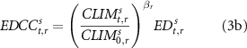
The approaches used to model the 'intensive margin' can be schematized in two different categories: (i) scaling factor; (ii) exogenous shift parameter. The 'scaling factor' approach involves including, in the energy demand function for the thermal adaptation service s in region r and with a time step of t(  ), a multiplicative term based on the level (equation (1a)) of the climate variable (
 ) or its relative increase with respect to the baseline year (
 ), equation (1b)):

or
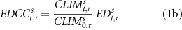
Where ED is the energy demand for the thermal adaptation service s( cooling or heating) without climate change and  is the energy demand for the thermal adaptation service under climate change.
The climate variables ( ) most commonly used to capture thermal stress are cooling degree days (CDDs) and heating degree days (HDDs). The CDDs (HDDs) are defined as the number of degrees above (below) the thermal comfort threshold, measured in terms of day count (ASHRAE 2017):
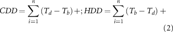
where '+' signifies only positive values that accumulate over n days in the chosen time period,  the daily mean outdoor air temperature and
  the threshold temperature. All the studies are reviewed by adopting the scaling factor set
  to 18 °C, while few of them evaluate alternative thermal comfort thresholds (Hasegawa et al 2016, Park et al 2018).
In some cases, the scaling factor includes an empirically estimated parameter  that modulates the proportional variation in the climate indicator, either in a linear (equation (3a)) or an exponential fashion (equation (3b)):
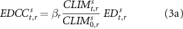
or
Equations (1a)–(1b) are the most commonly used approach that is found both in the engineering and end-use demand models—they add the scaling factor to the building energy consumption model (Labriet et al 2015, IEA 2018, Levesque et al 2018, Clarke et al 2018), and by energy system bottom-up analyses—they add the scaling factor to their stylized income–demand relationship (Isaac and van Vuuren (2009)), Mima and Criqui (2009), Hasegawa et al( 2016), Park et al( 2018). Equation (3a) is adopted by Tol (2013), while equation (3b) is adopted by Clarke et al( 2018).
The scaling factor method relies on the computation of CDDs and HDDs (equation (2)) from the historical and future mean air temperature. The increase in energy demand across different warming scenarios therefore will depend on two transmission mechanisms: (1) how mean temperature increases affect CDDs and HDDs; (2) how variations in the CDDs and HDDs affect the cooling and heating demand via the scaling factors (Equations 1 and 3). Therefore, if the relationship between mean temperature and degree days is non-linear (Mourshed 2012), the relationship between temperature and energy demand is also non-linear, even when models include a simple proportional factor between energy and degree days (equation(1a) and (1b)).
An empirical estimation of the non-linear transmission from temperature to degree days and energy demand is presented in figure 2. The estimated relationship is based on a pooled regression model between temperature, CDDs and HDDs (Panel a), computed with varying thresholds: 18 °C and 22 °C as for CDDs, 18 °C and 16 °C as for HDDs (equation (2)). Meteorological data is obtained from the NASA Earth Exchange Global Daily Downscaled Climate Projections (NEX-GDDP)5 dataset, for the years from 1986 to 2005. The left quadrants show the best fit (cubic) obtained from the regression model. A stylized relationship between the country-level, mid-century mean temperature shocks (temperature scale factor) and the shock on the CDDs and HDDs is assessed by computing the percentage variation of the mean future realization (mean of 2041–2060) with respect to the variables' historical level (mean of 1986–2005). The indicator corresponds to the shock of energy demand that models adopting the scaling factor would transmit on cooling and heating energy demand at the country-level. Results underscore that a given annual mean temperature percentage variation leads to a more-than proportional increase (decrease) in the CDDs (HDDs) percentage variation (as most observations fall above or below the bisector). Furthermore, the magnitude of the degree days' percentage variation associated to a given temperature shock increases sharply when the higher threshold for CDDs is adopted and in RCP 8.5, while the shock is more uniform across thresholds and climate scenarios as for HDDs.
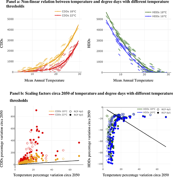
Figure 2. Panel a: Non-linear relationship between temperature and degree days with different thresholds. Panel b: Percentage variation of temperature and degree days circa 2050. Country level observations are constructed from the population-weighted aggregation of gridded data from NEX-GDDP. The left quadrant shows the best model fit of the yearly mean temperature on the degree days, between different polynomial specifications (linear, quadratic, cubic) selected on the basis of the lowest residual mean square error (RMSE) and the statistical significance of the coefficients. NEX-GDDP data of mid-21st century climate (2041 to 2060), under the RCP 4.5 and RCP 8.5 is used to compute the scaling factor of the country-level mean temperature, CDDs and HDDs circa 2050.
Download figure:
Standard image High-resolution imageThe 'exogenous shift parameters' approach varies key model parameters describing the efficiency of energy use and therefore, indirectly, of demand for energy, on the basis of parameters estimated empirically with historical data. This approach entails a different representation of the responses to weather shocks with respect to the 'scaling factor'. First, elasticities are differentiated by fuel type (typically oil, gas and electricity) rather than by end-user service. A fuel-specific coefficient provides a measure of the shock that compounds the contribution of different thermal adaptation services. Second, climate indicators used by empirical studies are more commonly mean temperature levels (De Cian et al 2013) or temperature bins (De Cian and Sue Wing 2019), rather than CDDs and HDDs. A V-shaped or a linear-spline response function of energy demand to climate (figure 3) makes it possible to associate the coefficients of low temperature levels or bins to heating requirements, while cooling needs are associated with the coefficients related to high temperature levels or bins.

Figure 3. Stylized V-relationship between energy demand and temperature.
Download figure:
Standard image High-resolution imageWithin this approach, a climate change impact shock Ψ for each fuel f, country c, and future time period t is obtained by combining the estimated coefficients  with exposure under historical (
 ) and future (
 ) climate (equation(4a)). The resulting shock is applied to energy demand without climate change (ED) to obtain demand with climate change (
 ):
):

Computable GE (CGE) models (Eboli et al 2010, Francesco Bosello et al 2012, Roson and Van der Mensbrugghe 2012) have used climate-induced shocks on energy demand, such as those estimated by De Cian et al( 2013),6 De Cian and Sue Wing (2019), or by van Ruijven et al( 2019) to calibrate the exogenous shifts in their models. It is important to distinguish between the empirical studies estimating those shocks, which are top-down PE studies that do not take price adjustments into account, and the CGE modeling studies, which are top-down assessments that explicitly account for GE adjustments. The parameter of the response of thermal adaptation to temperature ( ) can be estimated by using dynamic models (such as error correction models) that make it possible to identify long-term elasticities, combining the contributions of the intensive and extensive margins in a single parameter. In this manner, modeling studies using exogenous shifts calibrated on long-term elasticities implicitly account for the penetration of AC.
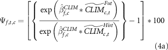
The extensive margin has been modeled through a market penetration model that explicitly estimates the market penetration of air-cooling appliances. Most studies (Isaac and van Vuuren 2009, Mima and Criqui 2009, Hasegawa et al 2016, Park et al 2018; Levesque et al 2018,7 Arnell et al 2019) rely on the two-stage penetration model by Mcneil and Letschert (2008, 2010) and Sailor and Pavlova (2003),8 in which Penetration (P) of air-cooling appliances is a function of two components: the Climate Maximum, CM( figure 4, panel a, left quadrant), which identifies the maximum share of AC adoption modulated by the climate conditions (measured by the CDDs) if no income constraint existed; and Availability, AV (figure 4, panel a, right quadrant), which identifies the share of the Climate Maximum which is actually achievable given the income level of the population (I). Penetration is defined as the product of these two components (figure 4, panel b).
A few studies rely on other approaches. IEA (2018) uses a 'stock model' approach. The modeling of penetration is based on the stock of cooling equipment that is necessary to meet the required energy service demand. Assumptions on average equipment lifetime are applied by using a Weibull distribution to determine the rate at which each equipment category diminishes over time. Annual sales volumes and corresponding energy performance assumptions are calculated with respect to remaining stock and energy service demand in a given year. Clarke et al( 2018) model the extensive margin as a unitless calibration coefficient, modulating the per capita energy service demand per unit of HDD/CDD and floorspace (a 'saturation parameter'). A narrow number of studies do not account for extensive margin developments (Tol 2013, Labriet et al 2015).
Figure 4. Calibration values of the AC Climate Maximum, Availability and Penetration functions.
Download figure:
Standard image High-resolution image3.3.2. Sectoral heterogeneity
Whether the way the transmission of climate shocks to thermal adaptation services across different sectors—residential and commercial—is represented in models varies across IAMs. As for the intensive margin, models that rely on the scaling factor assume that a given climate shock identically affects the response of the two sectors. In its most general formulation, the scaling factor approach makes it possible to disentangle the difference between residential and commercial short-term shocks, since a sector-specific modulation parameter can be included in the function. Nevertheless, in all cases analyzed this modulation parameter is either set to unity (Labriet et al 2015, Hasegawa et al 2016, Park et al 2018) or assumed to be constant across sectors (Clarke et al 2018). As for the extensive margin, the device penetration ratio obtained in the residential sector is generally used for the commercial sector (Hasegawa et al 2016, Park et al 2018). On the other hand, studies that model transmission via the 'exogenous shift parameters' adopt sectoral-specific parameters, such as the panel econometric models used for calibration estimate of the equations separately for each sector (De Cian and Sue Wing 2019).
3.4. Combined classification
Table 1 summarizes the resulting classification of the studies reviewed, based on the different modeling characteristics pertaining to the relationship between the economy and the energy system, its level of detail, breaking down the climate feedback of final use of energy into five overall model types. Type 1 models (bottom-up, PE models with a market penetration module for AC) have been adopted most frequently, followed by Type 3 (CGE coupled with a process-based representation of the energy sector and a market penetration module for AC) and Type 5 (top-down CGE simulation approaches deploying exogenous shifts) models. Type 2 models (top-down PE simulation approaches deploying exogenous shifts) have been adopted only by two studies, while Type 4 (CGE coupled with a process-based representation of the energy sector characterizing only the intensive margin) shows the contribution made by a single study. The comparison of consistent scenarios between Types 3 and 4 makes it possible to discern the effect of including the extensive margin in CGE. The comparison of consistent scenarios between Type 2 and Type 5 sheds light on the role of adaptive behaviors induced by changes in prices and interactions across markets.
4. Analysis of IAM projections
4.1. Projections: Global and regional trends in heating and cooling demand
Model results underscore that at the global level the increases in energy demand driven by higher cooling needs more than compensate for the decreases in energy demand due to lower heating needs. Figure 5 shows the distribution of the results obtained across different climate change scenarios (RCPs) for cooling services, heating services and combinations for all buildings and the residential sector only. Projections are reported for 2050 and 2100, in quantity (left quadrants) and in relative terms with respect to the demand in 2016 (right quadrants). The range in the projections expressed by the boxplots represents differences across models and socioeconomic scenarios (SSPs) in Panel a and Panel b, while differences across models and climate scenarios (RCPs) in Panel c. The projections point to an important increase in energy for thermal adaptation as the combination of cooling demand increases and heating demand decreases. The evidence of the increase (decrease) in cooling (heating) demand is consistent across warming scenarios and over time. Depending on the combination of service, sectors, and RCP scenarios, there are important differences in the magnitude of the projections. Uncertainty increases over time, especially in relation to cooling demand when commercial activities are also included. The boxplots show that the range of projection results is much wider for cooling demand than for heating demand and for total building demand than for residential demand. In the scenario assuming no variations in the climatic conditions, the median total demand for thermal adaptation increases up to 77 (85) EJ and by a factor of 1.30 (1.43) with respect to 2016 (59 EJ), in 2050 (2100). In the low warming scenarios, RCP 1.9 and RCP 2.6, the median total demand increases up to 92–96 (120–130) EJ and by a factor of 1.5–1.6 (2–2.2) in 2050 (2100). In the moderate warming scenario RCP 4.5 the median total demand increases up to 75 (115) EJ and by a factor of 1.26 (1.93) in 2050 (2100). In the high warming scenarios RCP 6 and RCP 8.5 the median total demand increases up to 73–97 (130–147) EJ and by a factor of 1.23–1.63 (2.2–2.47) in 2050 (2100). The heterogeneity across SSPs and IAM models is presented in Panel b. Median values of thermal energy demand exhibit moderate variability across SSPs especially for the residential sector and in the first half of the century. Differences across socio-economic scenarios are instead more evident in the building sector in 2100, for both cooling and heating demand. Overall, heterogeneity across scenarios is more marked when focusing on climate shocks of different magnitude (Panel a), than on socioeconomic scenarios (Panel b). This result points to the need for further investigation of the way in which different mechanisms of propagation between climate and energy demand can affect model projections.
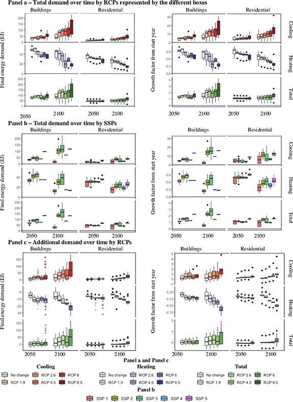
Figure 5. Energy demand boxplot across RCPs (panel a), energy demand boxplot across SSPs (Panel b), Energy demand, additional contribution due to climate change (panel c). Data reported in the boxplots is taken from: Labriet et al( 2015); IEA (2018); Levesque et al( 2018); Clarke et al( 2018); Isaac and van Vuuren (2009); Mima and Criqui (2009); Park et al( 2018); Arnell et al( 2019). Data points with the star marker refer to the results from van Ruijven et al( 2019). Different temperature change scenarios have been converted to RCP scenarios by using the median of each RCP range for 2080–2100 in IPCC (2014): 0.3 °C to 1.7 °C under RCP 2.6, 1.1 °C to 2.6 °C under RCP 4.5, 1.4 °C to 3.1 °C under RCP 6.0 and 2.6 °C to 4.8 °C under RCP 8.5. The 'No Change' scenario represents the cases in which current climate conditions (CDDs/HDDs) are assumed throughout the time period. Historical values for 2016 are computed by using data from IEA (2018) and Park et al( 2018).
Download figure:
Standard image High-resolution imageThe additional contribution of climate-induced shock on energy demand for thermal adaptation is obtained by computing the difference between the projected demand in a given RCP scenario and its counterpart in the 'no climate change' scenario, sharing the same socio-economic assumptions (SSPs). This approach makes it possible to single out the climate transmission effect from the impact of socio-economic trends (Panel c). The studies included in Panel c correspond to the one included in Panels a and b, with the addition of the projections by van Ruijven et al( 2019). The latter are singled out (highlighted as an asterisk) and are not used to compute the distribution of the boxplots, to ease the comparison between Panel a and c, as this study only provides results in terms of the additional contribution due to climate change.
As for cooling, the climate change-induced median variations in energy demand for the building sector range from 4 EJ to 17 EJ (from 20 EJ to 84 EJ) in 2050 (2100), depending on the climate scenario. As for heating, the climate change-induced median variations in energy demand for the building sector range from −4 EJ to −11 EJ (from −4 EJ to −23 EJ) in 2050 (2100), depending on the climate scenario. Thermal adaptation in buildings is projected to require additional energy ranging from a median value of 0.01 EJ (16 EJ) under the RCP 1.9 and to 8.5 EJ (61 EJ) under the RCP 8.5 in 2050 (2100). Current energy usages amount to 52 EJ for heating and 7 EJ for cooling, for a total of 59 EJ, in buildings, and to 39 EJ for heating and 3 EJ cooling, for a total of 42 EJ, in the residential sector. Even in the low warming scenarios, RCP 1.9 and RCP 2.6, net final demand goes up by a median value of 16–22 EJ in 2100, though a net reduction cannot be excluded. The realization of a very low warming scenario, RCP 1.9, with respect to the RCP 2.6, would reduce the median net final demand by 3.7 EJ (6 EJ) in 2050 (2100), that is by 6% (10%) of net final demand in 2016. The commercial sector accounts for the largest share in the incremental contribution of climate change to energy demand, as specific projections of residential sectors show that the additional demand required ranges from −2 EJ to −0.5 EJ (from 1.4 EJ to 14 EJ) in 2050 (2100).
The relative importance of the climate change-induced variations in the energy demand for residential buildings, with respect to the no-climate change scenario, are amplified at the regional level (figure 6). All macro regions are characterized by a net increase of a building's energy demand for thermal adaptation, ranging from 0.5 to 7 EJ in 2050 and from 6 EJ to 23 EJ in 2100, depending on the region and the degree of warming. Sharp increases in median additional energy due to cooling requirements from 2050 to 2100 are projected for all regions, with a median addition in Asia, the Middle East and Africa (MAF) and OECD countries between 23 EJ and 28 EJ under the highest warming scenarios. As for the residential sector, the median additional energy due to cooling requirements in 2100 ranges from 1.9 EJ to 8.7 EJ in Asia, from 1.4 EJ to 9.1 EJ in MAF, from 0.3 EJ to 2.4 EJ in OECD countries, from 0.3 EJ to 1.7 EJ in Latin America (LAM) and from 0.02 to 0.3 in Russia (REF), depending on the RCP. In temperate regions, OECD and REF, sharp decreases in heating energy needs result in a median value of total additional energy requirements in 2100 which ranges from −1.1 to −3.6 in the former and −0.3 and −0.9 in the latter region, depending on the RCP. On the other hand, in Asia and MAF the total energy requirements range in 2100 from 0.5 to 4 EJ (an almost tenfold increase from RCP 1.9 to RCP 8.5) in the former region and from 1 EJ to 6 EJ in the latter. In LAM total additional demand goes from almost zero to 1 EJ. The additional energy demand projected in higher warming scenarios, with respect to the low warming scenarios, is greatly amplified from the second half of the century in both the residential and the commercial sector.

Figure 6. Additional demand over time by world region. Additional contribution due to climate change in value in five world macro-regions in the buildings (Panel a) and residential (Panel b) sectors. Results are grouped by RCP scenarios. Studies in Panel a: Park et al( 2018); Studies in Panel b: Park et al( 2018); Arnell et al( 2019). Regional results from van Ruijven et al( 2019) are not reported for clarity but a graph with those results is available upon request. van Rujiven's estimates for cooling demand in buildings in circa 2050 reach 55, 12, 50 EJ (22, 5, 21 EJ) in Asia, MAF, OECD, respectively, under the RCP 8.5 (RCP 4.5). Heating estimates reach −6 and −12 EJ (−4 and −9 EJ) in Asia and OECD, respectively, under the RCP 8.5 (RCP 4.5).
Download figure:
Standard image High-resolution imageGlobal and regional trends in heating and cooling demand are assessed with respect to the most common drivers modeled by IAMs: climate and GDP. Other key cooling and heating demand drivers, namely building characteristics (floor space, insulation properties), appliance characteristics (HVAC system type and efficiency) and behavioral aspects (thermal comfort thresholds, energy saving behaviors), could not be investigated in similar detail. The IAMs incorporating bottom-up technology rich modules (building or energy system models) or flexible end-use functions (energy demand models) account for such drivers by including building characteristics (generally floor space) and HVAC system efficiencies (generally the energy efficiency ratio, or EER). Usually, the positive correlation between floor space and GDP is used to model the evolution of this variable over time. Some studies simulate different behaviors of people towards the use of AC by varying the temperature thresholds used to compute CDDs and HDDs across SSPs (Hasegawa et al 2016, Levesque et al 2018, Park et al 2018). Even when building and behavioral characteristics are taken into account, the marginal contribution of such drivers is often hidden in model results and projections are presented in an aggregate way that does not permit a direct comparison between those different assumptions. Based on the results gathered, it was possible to elaborate only on the role of HVAC system efficiency by by relying on Isaac and van Vuuren (2009) and IEA (2018), which investigate the extent to which the energy efficiency of heating and cooling appliances influence space cooling energy needs. Table 2 summarizes the main assumptions and key results: higher appliance efficiency brings cooling energy demand down by 30% in 2050 (IEA 2018) and by 45% in 2100 (Isaac and van Vuuren 2009), while heating demand would be more than halved in 2100 (Isaac and van Vuuren 2009).
Table 2. IAM-based studies assessing the impact of appliance efficiency on projections of energy demand.
| Model | Study | Sector | Assumptions of the efficiency scenario | Reduction of energy demand (% decrease) from baseline at the end of the time horizon |
|---|---|---|---|---|
| TIMER IMAGE | Isaac and van Vuuren (2009) | Residential | Heating: shift from electrical resistance heating to more efficient heat pumps. Cooling: Increase in the energy efficiency ratio (EER) from 2.4 EER to 6.32 (4.39 in the baseline). | Heating: reduction of 17 EJ in 2100 (−56%) Cooling: reduction of 15 EJ in 2100 (−30%) |
| IEA ETP | IEA (2018) | Buildings | Cooling: efficiency is 50% higher in 2030 and 80% higher in 2050 than in the baseline scenario. | Cooling: reduction of 10 EJ in 2050 (−45%) |
4.2. Importance: Implications for the economy, and the environment
With respect to the economic implications, most CGE-based studies underscore that, since energy is only a small part of the overall macroeconomic inputs, climate-induced impacts on energy demand have little economic repercussion; such repercussions are mainly driven by impacts on the agricultural sector, sea level rise, health and tourism impacts. Figure 7 presents the results of the climate-related impact on GDP due to variations in energy demand for cooling and heating as a response to global warming. Substantial impacts are identified under the RCP 8.5 scenarios, with a median relative variation in GDP equal to −0.29%, with the lowest value reaching −1.9%. The projections based on the SSP 1 are characterized by a positive median GDP percentage change of relatively small magnitude,9 while a negative median GDP percentage change is found in the projections based on SSP 2 and SSP 3.
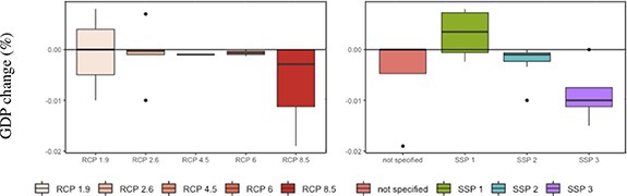
Figure 7. Economic implications of impacts of energy demand.Percentage GDP variation in 2100 across RCPs (left) and SSPs (right) relative to the 'no climate change' scenarios. Total number of scenarios: 19. Boxplots represent the heterogeneity across different studies: Park et al( 2018); Hasegawa et al( 2016); Roson and Van der Mensbrugghe (2012); Tol (2013); Francesco Bosello et al( 2012); Eboli et al( 2010). Different temperature change scenarios have been converted to RCP scenarios by using the mean of each RCP range for 2080–2100 in IPCC (2014): 0.3 °C to 1.7 °C under RCP 2.6, 1.1 °C to 2.6 °C under RCP 4.5, 1.4 °C to 3.1 °C under RCP 6.0 and 2.6 °C to 4.8 °C under RCP 8.5.
Download figure:
Standard image High-resolution imageWhile early studies generally found a very limited macroeconomic impact in terms of welfare change at the global level, a more recent analysis has identified a higher role of the energy demand with respect to the macroeconomic impacts of climate change. Francesco Bosello et al( 2012), Roson and Van der Mensbrugghe (2012) and Dellink et al( 2014), Labriet et al( 2015) find negligible impacts of changes in energy demand due to HDD and CDD variations. Tol (2013), using the FUND model, finds that the negative impact of the net increase in energy demand is quantified as a variation of −1.9% of GDP by 2100. In contrast to the previous studies, Hasegawa et al( 2016) and Park et al( 2018) include the incremental costs for investments in cooling technology on top of the welfare changes due to the variations in energy demand and find negative median impacts on GDP in 2100, ranging from −0.94% under the RCP 8.5 to −0.05% under the RCP 1.9.
At the regional level, these studies highlight the role of terms-of-trade as a driver of GDP changes. The economy will be negatively affected in fossil-fuel-exporting countries, as they experience a reduction in the demand for their exports due to the reduction in heating service, while fossil-fuel-importing countries will benefit from the decrease in heating expenses. In some cases, these welfare mechanisms are moderated by the rebound effects generated by the changing fuel prices, as shown by Labriet et al( 2015). The study is the only IAM-based assessment accounting for price-induced rebound effects on consumption. GE gas consumption for heating is higher than what is found in the PE. The price change deriving from the decrease in gas consumption for heating impacts the energy markets through rebound effects that, globally, result in a less sharp decrease in the demand for heating energy (the ex-post percentage decrease is 34.2%–38.3% higher than the initial projections, depending on the long-term temperature increase going from 1.6 °C to 5.7 °C).10
The few studies reporting the impact of thermal adaptation on global emissions with respect to the emissions in the no climate change scenario tend to find only marginal impacts. Labriet et al( 2015) quantify the total emissions from the increase in energy demand for buildings in 2100 to be 1.2 (2.5) Gt CO2/year under RCP 6 (RCP 8.5), while Isaac and van Vuuren (2009) find an increase related to residential energy demand of 1.17 Gt CO2/year under RCP 8.5. The feedback between the energy and climate systems due to changes in heating and cooling services at the global level should not be considered negligible even if the overall magnitude of the increase is low. Moreover, it is important to keep in mind that these two studies might underestimate the needs of energy for adaptation because the extensive margin is not modeled (Labriet et al 2015) or because the commercial sector is not included (Isaac and van Vuuren 2009).
4.3. Sources of variation
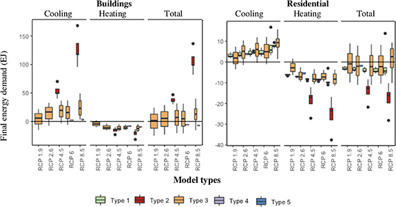
Notwithstanding the robust general trends with respect to heating and cooling demand, model results show significant heterogeneity. Figure 8 presents a disaggregation of the incremental energy demand projected by different IAM categories (Types 1–5), for residential (left quadrant) and buildings (right quadrant). Only part of the groups identified provide projections in each combination of year (2050 and 2100), energy service (cooling, heating and combined) and sector (residential, buildings). Therefore, only the projections which make it possible to simultaneously compare the highest number of groups are included, namely the projections reporting the value of the incremental energy demand in 2050.
Figure 8. Additional contribution due to climate change in 2050 by model types. Left quadrant: building (commercial and residential) sector. Right quadrant: residential sector. Type 1 models: TIMER-IMAGE; POLES. Type 2 models: projections from van Ruijven et al( 2019). Type 3 models: AIM/CGE, GCAM. Type 4 models: TIAM WORLD GEM-E3. Type 5 models: ICES.
Download figure:
Standard image High-resolution image
The analysis of the projections reported in figure 8 suggests that models lacking extensive margin adjustments (Type 4) highly underestimate the additional cooling needs of the building sector, finding an overall reduction in energy demand. Instead, the requirements for heating are in line with other modeling approaches. This result points to the importance of including the extensive margin in the structure of IAMs energy demand. Other major modeling differences are ruled out, as Type 4 models differ from Type 3 models only as regards their representation of the extensive margin.
There is no univocal relationship between the results of projections and the modeling of the interactions between the economy and the energy system. Among the processed-based, bottom-up models, PE IAMs (Type 1) tend to project a median energy increment in line with the level projected by those GE IAMs adopting the same type of modeling of climate shock (Type 3). Scenarios from Type 1 models show a much smaller dispersion compared to Type 3. Type 1 models—bottom up models—might be more optimistic regarding the role of technological change and efficiency improvements compared to Type 3 models.
Among the top-down simulation models relying on exogenous shifts, PE IAMs (Type 5) tend to project a higher median increment than GE IAMs (Type 2) and a higher median reduction. Type 2 models do not include the important effect of prices, which are also related to the net trading position on the international market (terms of trade effect). Higher prices would induce a partial reduction in demand. Lower prices could induce a rebound effect, pushing further demand. GE effects also imply changes in the income available to households and in the cost structure of producers, which are further elements that can lead to differences between PE and GE effects.
The intensity of future global warming exacerbates the differences across model type results. For instance, in the projections of the total incremental demand of buildings (Panel a), under RCP 4.5 (RCP 8.5), the median total demand of Type 2 models is two times (five times) higher than the median demand of Type 3 models. This pattern is consistent across end uses and sectors, and suggests that the specific choice over the climate variable and the functional form of climate shock may affect the projections more sharply than other modeling aspects.
The differences across the projections of model types vary according to the specific sector and end use service. The gap between the projections is higher than for the cooling demand of the commercial sector (panel a) and for the heating demand of the residential sector (panel b). Top-down models based on sectoral-specific exogenous shift parameters project substantially higher increases in incremental commercial cooling demand. Energy demand for the residential sector projected by Type 2 top-down models (van Ruijven et al 2019) and by Type 3 models (GCAM by Clarke et al 2018 and AIM/CGE by, Park et al 2018) under the SSP 2 and RCP 8.511 is comparable (8 EJ in the former study and 9–10 EJ in the two latter studies), while it differs remarkably when the commercial sector is considered (114 EJ in the former study and 4–22 EJ in the two latter studies). Therefore, the adoption of transmission mechanisms of climate on energy demand allowing for the sectoral characterization of the shocks can be identified as a key driver of heterogeneous results.
5. Discussion and concluding remarks
The relationship between energy demand and the climate system is bilateral. Energy demand, for centuries met from the combustion of fossil fuels, has been and still is a primary source of greenhouse gas emissions. At the same time, energy is a key input to resilience, as several energy services make it possible to maintain conditions of thermal comfort across all sectors of the economy under varying weather and climate conditions. No inquiry has been made about the extent to which adaptation to climate change might further feed into the energy and socio-economic system by requiring more energy, and therefore initiate a negative feedback loop. How such an interaction actually plays out varies across regions, and depends on the configuration of the energy system, socioeconomic development, and local climate. Answering this question requires the development of Integrated Assessment Models that integrate climate impacts and policies in a consistent manner, bringing together two research communities that have traditionally worked in parallel.
This paper systematically reviews and compares quantitative projections of energy demand in commercial and residential buildings that include additional energy use or savings induced by thermal adaptation to heating and cooling needs at global and regional levels. Despite the huge number of scenarios generated by the IAM community, only 14 studies (leading to 69 energy scenarios and 19 macroeconomic scenarios, for a total of 88) that project energy demand under different socio-economic and climate scenarios and that account for the feedback from the climate into energy demand could be identified. The resulting studies are analyzed based on a classification that considers in detail the energy system, the relationship between the energy and the economy, and the technical representation of the specific demand for heating and cooling.
Results show that projections underestimate the energy demand of the building sector when energy use is driven solely by income and population drivers and not by changing climatic conditions and subsequently by rising adaptation needs. The analysis provides substantial evidence of an increase (decrease) in cooling (heating) demand across warming scenarios and over time. However, there are, depending on the combination of service, sectors, and RCP scenarios, important differences in the magnitude of the projections. Uncertainty increases over time, especially in relation to cooling demand and when commercial activities are included. Thermal adaptation in buildings due to climate change is projected to require additional energy, ranging from a median value of 0.01 EJ (16 EJ) under the RCP 1.9 to 8.5 EJ (61 EJ) under the RCP 8.5 in 2050 (2100), corresponding to a 2% (11%) increase under the RCP 1.9 and a 13% (70%) increase under the RCP 8.5, with respect to future demand under no climate change in 2050 (2100). The projected additional median demand in buildings required in 2100 under RCP 8.5 corresponds to a doubling with respect to total building demand in 2016.
Models lacking extensive margin adjustments highly underestimate the additional cooling needs of the building sector. Two main archetypes of extensive margin modeling are identified, and they are either based on a weak empirical basis (the market penetration approach) or they only implicitly account for the future evolution of air-conditioning ownership (the exogenous shift approach). Recent country-specific studies have highlighted the amplification effect deriving from the growth in appliance ownership in Mexico (Davis and Gertler 2015) and in California (Auffhammer et al 2017), while Pavanello et al( 2019) suggest that a much richer set of socio-economic, demographic, and behavioral factors influences the diffusion of air-cooling appliances.
Future research aimed at deepening the integration of climate impact feedback into the mitigation and energy scenario needs to address two challenges. First, to what extent the empirical basis concerning the adoption and use of energy-using durables particularly sensitive to climate and weather conditions, such as air conditioning, will extend to countries where those dynamics have not been investigated. Second, how to use the new emerging evidence across multiple countries, regions, and sectors, often by means of different methods, to better represent the climate-energy feedback loop in IAMs in a consistent way while avoiding double counting. Our review has also highlighted the much larger uncertainty that characterizes the commercial sector, which, due to the lack of sector-specific data or evidence, is modeled similarly to the residential sector (table 3), while empirical results suggest that the response to changes in temperature can vary greatly across sectors (De Cian and Sue Wing 2019).
Table 3. Feedback between energy demand and climate: frequency of different characteristics.
| N° of studies | ||
|---|---|---|
| Intensive margin modeling | Exogenous shift parameter | 5 |
| Scaling Factor | 9 | |
| Extensive margin modeling | Market penetration | 8 |
| Exogenous shift parameters | 5 | |
| Not modeled | 1 | |
| Functional form across sectors | Homogeneous | 6 |
| Heterogeneous | 1 | |
| Only one sector considered | 7 | |
| Functional form across world areas | Homogeneous | 9 |
| Heterogeneous (e.g. temperate vs tropical countries; climate clusters) | 5 | |
| Climate variable adopted | CDDs/HDDs | 9 |
| Temperature | 4 | |
| Temperature bins | 1 | |
| Extreme events (e.g. heat waves) | 0 |
Note: Intensive and extensive margin modeling: classification of modeling approaches developed in order to include short-term and long-term climate-induced shocks on cooling and heating energy demand, as identified in section 3.3. Functional form across sectors: how the intensive or extensive margins are modeled and parameterized in the commercial and residential sectors (if homogeneous, no difference is allowed in the calibration of the function parameters for different sectors). Functional form across world areas: how the intensive or extensive margins are modeled and parameterized across different regions (if homogeneous, no difference is allowed in the calibration of the function parameters for different regions). Climate variable adopted: which climate variable is included in the intensive and extensive margin formulas.
IAMs have paid scarce attention to the nonlinear responses of energy demand to extreme events, such as heat waves (table 3). A major challenge derives from the different time scale of CGE and bottom-up engineering IAMs, which typically run with yearly time-steps (Ciscar and Dowling 2014). In order to effectively capture the impacts of future extremes, new empirical studies would need to adopt datasets that are rich in terms of spatial and temporal resolution, with weather observations and energy data processed and aggregated in a way that preserves information regarding the tails of the weather distribution and its geographical specificity. Unless the short-term elasticities of demand are calculated at the same temporal and spatial scale as the IAM simulations into which they will be incorporated, the aggregation of short-term elasticities for the adoption in IAM is an important methodological limitation (Sue Wing and Lanzi 2014). Stochastic modeling techniques and model-integration would need to be used in order to capture short-term events, an approach adopted so far mostly at the regional level, as by the Platform for Regional Integrated Modeling and Analysis developed by the Pacific Northwest National Laboratory (Kraucunas et al 2015) or the Global Assessment Modeling Framework developed by the International Institute for Applied Systems Analysis (Huppmann et al 2019). Aggregation of regional elasticities implies that several regions are forced to have similar temperature responses, although final demand shocks would differ among regions because future changes in temperature vary geographically. Developing IAMs capable of characterizing the sub-national diversity of heating and cooling needs is certainly warranted.
Acknowledgments
This research has received funding from the European Research Council (ERC) under the European Union's Horizon 2020 research and innovation programme under grant agreement No 756194 (ENERGYA). The authors would like to thank the organizers of the EAERE—CD-LINKS Summer School on Integrated Assessment Models for very helpful comments and suggestions. We are grateful to Chane Park and Fujimori Shinichiro for providing results from their models that have been included in the Review.
Data availability statement
All data that support the findings of this study are included within the article (and any supplementary information files).
Footnotes
- 4
Table 1 in Supplementary Materials presents the number of documents resulting from the different searches. The search terms used for the meta-analysis included 'energy demand' OR 'energy use' OR 'energy consumption' AND 'climate change' AND 'conditioning' OR 'cooling' AND 'heating'. Other terms were progressively added to refine the search, such as AND ('GDP' OR 'wealth' OR 'economic loss' OR 'economic gain'); AND ('scenario' OR 'projection' OR 'impacts'); AND ('integrated assessment model' OR 'energy model)'.
- 5
NEX-GDDP is a large ensemble of downscaled and biased-corrected 0.25 gridded daily meteorological fields from 21 Global Climate Models (GCMs) that simulate vigorous (RCP 8.5) and moderate (RCP 4.5) warming under the Coupled Model Intercomparison, Phase V (CMIP5) climate model exercise. https://cds.nccs.nasa.gov/nex-gddp/.
- 6
De Cian et al( 2013) assess the climatic impact on the demand for electricity and for three different types of fuel, gas and oil products, by using a world panel of 31 countries. Temperature variations are segmented by using seasonal (spring, fall, summer and winter) temperatures. Geographical variability is taken into account by introducing climatic clusters among countries. In particular, De Cian et al( 2013) group the countries into three clusters. The authors find for instance that, for electricity, the short-term effect of summer temperature is significant in all groups, but with a different sign. In very cold countries a 1% increase in summer temperature reduces annual demand by 0.51%. In very hot countries it increases electricity demand by 1.66%. In mild countries the increase in electricity demand is lower, equalling 0.54%. The authors find the same direction of short-term variations but coefficients of a bigger magnitude.
- 7
- 8
As for the Climate Maximum, Sailor and Pavlova (2003) and Mcneil and Letschert (2008, 2010) are based on data from 40 US cities (figure 4, panel a, left quadrant). The estimated equation is applied to all world regions by IAM-based studies on the assumption that penetration levels in the US have been unconstrained by income considerations and can therefore be considered as the upward threshold of penetration under a given climate condition. As for the 'availability' relation, the two empirical evaluations conducted, by Isaac and van Vuuren (2009) and by Mcneil and Letschert (2008, 2010), are based on the same cross-section dataset of 24 countries provided by McNeil and Letschert (2010). Most IAM-based studies (Mima and Criqui 2009, Hasegawa et al 2016, Park et al 2018, Arnell et al 2019) follow Mcneil and Letschert (2008, 2010)) for the Climate Maximum and Isaac and van Vuuren (2009) for the Availability calibration, resulting in AC appliance penetration levels varying in relation to both CDDs and income (figure 4, Panel b).
- 9
The gain appears only in Park et al( 2018) when they run the SSP 1 for 1.5 and 2 °C scenarios. The result could be due to basic differences in economic (GDP) and demographic assumptions; HDD/CDD threshold and differences in the assumption of annualized technological investment cost (Park et al 2018). Under SSP1 the study assumes a threshold for HDDs/CDDs equal to 15 °C/26 °C. For these assumptions heating reductions overcompensate cooling increases. In fact, energy demand decreases with respect to the no climate change scenario in Park's SSP1 1.5/2 °C scenarios.
- 10
The most affected regions are Europe, China, the USA, Canada and the former Soviet Union, as these regions experience higher absolute long-term variations in HDD. As for cooling, general equilibrium electricity consumption is lower than partial equilibrium calibration. The rebound effect induced by electricity prices results in a less sharp increase in energy demand for cooling (the ex-post percentage increase is 37.5%–42.4% lower than the initial projections, depending on the long-term temperature increase). The most affected regions are Europe, the USA, Canada and the Middle East. In Europe prices would increase by a range between 35% and 66% at the end of the time horizon, depending on the climate scenario, while in China and India prices would increase up to 30% and 55%, respectively, in the warmest months.
- 11