


Abstract
The b value of the Gutenberg–Richter (GR) distribution is estimated as a function of a threshold magnitude mth and it is found to depend on mth for magnitudes larger than the completeness magnitude mc. We identify a magnitude interval [mc, mm] where b is a decreasing function of mth followed by a regime of increasing b for large magnitudes. This is a common feature of experimental catalogues for different geographic areas. The increase at large mth is explained in terms of an upper magnitude cut-off in experimental catalogues due to finite size effects. We develop a rigorous mathematical framework to relate the decrease of b in the intermediate regime to the functional form of the distribution of the b values. We propose two hypotheses: The first is that the spatial and temporal variability of b leads to a b distribution peaked around its average value. The second is that main shocks and aftershocks are distributed according to the GR law with different b values, leading to a bimodal distribution of b. Simulated Epidemic Type Aftershock Sequences catalogues, generated according to this hypothesis, exhibit the same magnitude distribution of experimental ones. In alternative, we cannot exclude the b dependence on m caused by magnitudes not homogeneously evaluated in a seismic catalogue. In the latter scenario our results provide the correction terms to the estimated magnitudes.
1 INTRODUCTION
The Gutenberg–Richter (GR) law states that earthquake magnitudes are distributed exponentially (Gutenberg & Richter 1944) as Log10N(m) = a − bm, where N(m) is the number of earthquakes with magnitude larger or equal to m, b is a scaling parameter and a is a constant. The GR law is assumed to be the expression of earthquake self-similarity. Indeed the logarithmic relationship between the magnitude and the energy released by earthquakes (Kanamori & Anderson 1975) leads to a power-law distribution for earthquake energy, a signature of the absence of a characteristic scale in earthquake occurrence. Estimation of the b value is crucial for evaluation of the earthquake occurrence probability and justifies the large amount of literature on the issue. In general b assumes values very close to 1, although fluctuations (up to 30 per cent) around this typical value are observed depending on the catalogue, the estimating method and the magnitude range (Frolich & Davis 1993). Many authors have investigated the spatial variability of b (Ogata & Katsura 1993; Okal & Kirby 1995; Mori & Abercrombie 1997; Wiemer & Wyss 1997; Wyss et al.1997; Wiemer & Wyss 2002; Tormann et al.2014, and references therein) or its temporal variations (Imoto 1987; Jin & Aki 1989; Ogata & Abe 1991; Henderson et al.1992). Many mechanisms have been proposed to account for the observed spatial and temporal variability of b ranging from the fracturing degree and the material properties to the stress concentration degree, pore-fluid pressure or the focal mechanisms, including biases in the statistical estimation of b (King 1983; Utsu 1999; Amitrano 2003; Schorlemmer et al.2005). On the other hand, some authors proposed that the b value for tectonic earthquakes does not differ significantly from a universal value. This opinion was derived from the observation that the distribution of the seismic moment, whose logarithm is proportional to the magnitude, is very stable in space and time (Kagan 1997; Godano & Pingue 2000).
In this paper, we show that log N(m) versus m exhibits systematic deviations from the straight line predicted by the GR relation, indicating that the b value is not constant but depends on the lower magnitude threshold mth. In particular, we observe three different regimes: (1) for mth < mc, b is an increasing function of mth, (2) for mm > mth > mc, b is a decreasing function of mth and (3) for mth > mm, b is a slightly increasing function of mth. The behaviour in the first regime is largely expected and is attributed to catalogue incompleteness (Mignan & Woessner 2012, and references therein). Indeed for m < mc many events are not recorded and earthquake catalogues result incomplete for this magnitude range. In order to model this deviation Mignan (2012) proposed a multiplicative exponential term, interpreting the convex shape of the GR distribution as a consequence of the spatial variability of mc.
The behaviour in regime 3 can be attributed to the presence of an upper magnitude cut-off, mu. This regime has been previously observed and several equations have been suggested to reproduce such behaviour. In particular, it has been proposed that b assumes two different values depending on the m range (Pacheco & Sykes 1992; Okal & Romanowicz 1994; Sornette et al.1996), or else the GR relation has to be modified into a more complex functional dependence (Utsu 1971, 1978, 1999; Purcaru 1975; Caputo 1976; Vere-Jones 1976, 1977; Lomnitz-Adler & Lomnitz 1979; Kagan & Knopoff 1984; Main & Burton 1984; Olsson 1986; Kagan 1997).
More intriguing is regime 2 that cannot be simply explained. Here we show that the decreasing of b with mth is expected in all cases if b does not assume a single value but is distributed according to ϕ(b). In particular, we show that in the case that ϕ(b) is a narrow distribution centred at a characteristic value 〈b〉, it is possible to relate the functional dependence of b on mth to the functional form of ϕ(b). We also explicitly consider a bimodal ϕ(b) corresponding to the hypothesis that main shocks and aftershocks have two distinct b values. This hypothesis has been validated by means of numerical simulations of the Epidemic Type Aftershock Sequences (ETAS) model (Zhuang et al.2004), which also support the explanation of regime 3 in terms of finite size effects.
2 THE b VALUE VARIABILITY
We analyse six seismic catalogues: Southern California (SC) (Shearer et al.2005), Northern California (NC) (Waldhauser & Schaff 2008), Greece (Gr), Japan (Jp), Italy (It) and Switzerland (CH). Catalogue information, including temporal duration, geographic coordinates and number of events in each catalogue are reported in Tables 1 and 2.
The analysed data sets, the catalogue time period ΔT, the geographic extension and the number of events in the catalogue N.
| Catalogue | ΔT | Latitude N | Longitude W | N |
|---|---|---|---|---|
| SC | 1984/01/01 ÷ 2002/12/31 | 31.47 ÷ 37.03 | –121.51 ÷ −114.04 | 289385 |
| NC | 1984/01/01 ÷ 2005/12/31 | 35.30 ÷ 42.45 | –126.00 ÷ −116.34 | 298551 |
| Gr | 2003/01/01 ÷ 2012/07/01 | 33.10 ÷ 43.68 | 14.81 ÷ 35.03 | 90255 |
| Jp | 1985/07/01 ÷ 1996/12/31 | 25.73 ÷ 47.96 | 128.02 ÷ 148.00 | 159346 |
| It | 2005/04/16 ÷ 2012/05/23 | 35.00 ÷ 47.99 | 6.03 ÷ 18.98 | 85772 |
| CH | 1991/01/01 ÷ 2008/12/31 | 45.40 ÷ 48.30 | 5.60 ÷ 11.10 | 9728 |
The website where catalogues can be downloaded.
The website where catalogues can be downloaded.
To determine the variability of b with m we have adopted the method introduced by Cao & Gao (2002) to estimate mc, namely we evaluate the b value as a function of the cut off magnitude threshold mth. The b values are obtained by means of the maximum likelihood estimation (Aki 1965), |$b=\frac{{\rm Log_{10}(e)}}{\langle m\rangle -(m_c-\frac{\Delta m}{2})}$|, where 〈m〉 is the average magnitude and Δm = 0.1 is the magnitude binning. This last term has been added to the original Aki's formula for a more accurate b estimation (Utsu 1965; Guo & Ogata 1997). The uncertainty on the estimated b values is evaluated as |$\delta b=2.3 b^2\frac{\sigma _m}{\sqrt{N(m_{\rm th})(N(m_{\rm th})-1)}}$| (Shi & Bolt 1982), where σm is the standard deviation of the magnitude and N(mth) is the earthquake number with m > mth. We have checked that by applying a more accurate bootstrapping procedure (Amorèse et al.2010), our results are not significantly affected.
The b values as a function of mth are reported in Fig. 1. All six catalogs exhibit the regimes 1 and 2 described in the introduction, although for Italy the variations of b with mth are not very pronounced. Regime 3 is clearly observed for Greece, Japan and Switzerland. As discussed previously, regime 1 is largely expected and is attributed to catalogue incompleteness. Therefore we interpret the mth value, for which b is maximum, as the catalogue mc (values are reported in Table 3). The existence of regime 2 is further confirmed by stacking all catalogues and repeating the analysis for the new variable m1 = m − mc, with m ≥ mc. We obtain a clear decrease of b for small mth and a slow increases for larger mth (Fig. 2). The stacking procedure of all six catalogues reduces the uncertainty and makes deviations from a constant b more evident.
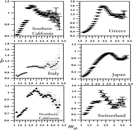
The b values as a function of mth for the six analysed catalogues.
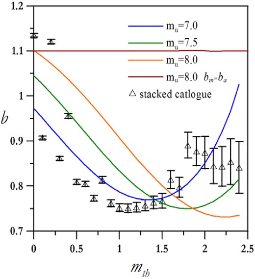
The b values as a function of mth for the stacked catalogues with the magnitudes shifted by mc. The continuous lines are b(mth) from the ETAS simulation with bm < ba (see text for details) and for different values of the cut-off magnitude mu. The horizontal ruby red line is b(mth) for the ETAS simulation with bm = ba (see text for details).
The completeness magnitude, 〈b〉 and the estimated parameters, γ and σ for the analysed catalogues.
| SC | NC | Gr | Jp | It | CH | ||
|---|---|---|---|---|---|---|---|
| mc | 2.5 | 2.7 | 3.3 | 3.6 | 2.2 | 2.2 | |
| 〈b〉 | 1.13 | 1.06 | 1.58 | 0.95 | 1.01 | 1.39 | |
| σ | 0.12 ± 0.03 | 0.12 ± 0.04 | 0.38 ± 0.16 | 0.13 ± 0.17 | 0.05 ± 0.03 | 0.27 ± 0.12 | |
| γ | 1.81 ± 0.01 | 1.79 ± 0.01 | 1.72 ± 0.01 | 1.78 ± 0.01 | 2.42 ± 0.99 | 3.06 ± 0.04 |
3 THE b DISTRIBUTION
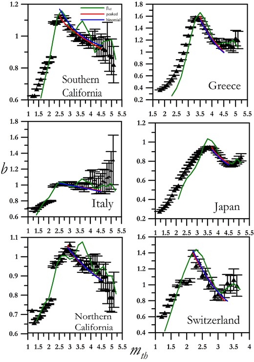
The b values as a function of mth for the six analysed catalogues compared to the beff (green line) values obtained numerically deriving the GR law. Red and blue lines are the best fit in regime 2 according to eqs (5) and (6), respectively.
In the following, we show that by assuming reasonable distributions for ϕ(b) we can obtain good fits for b(m).
3.1 Continuous peaked distributions
This result is intriguing since it allows to obtain information on the functional form of ϕ(b) from the dependence of b on mth. In particular the values of γ and σ can be obtained from the best fit of experimental observations (continuous red lines in Fig. 3) setting 〈b〉 = b(mth = mc). The estimated values of γ and σ are reported in Table 3 for the different catalogues here analysed.
For four catalogues γ ≃ 1.8 indicating that ϕ(b) is less steep, although not very different, than a Gaussian distribution. Whereas for Italy and Switzerland catalogues γ > 2.
3.2 Bimodal distribution of b
The b dependence on mth can be also interpreted in terms of a discrimination on the basis of the triggering mechanism, for instance supposing that main shocks are distributed according to a b smaller than the aftershock one. Indeed Bottiglieri et al. (2009) observed that a declustered Californian catalogue exhibits a b value smaller than the whole catalogue. To better check this point we apply a declustering procedure to experimental catalogues in order to separate aftershocks from background seismicity. More precisely, we use a space–time window declustering algorithm (Felzer & Brodsky 2006) according to which an event is identified as a main shock if a larger earthquake does not occur in the previous y days and within a distance |${\cal L}$|. In addition, a larger earthquake must not occur in the selected area in the following y2 days. We use typical values |${\cal L}=100$| km, y = 3 and y2 = 0.5. We then separately evaluate b as function of mth for the subset of events identified as aftershocks, ba, and as main shocks, bm. For all considered catalogues and for all values of mth, we systematically find ba > b > bm except for the Japan catalogue where ba < bm ≃ b for mth > 4.5 (Fig. 4). We wish to stress that the declustering technique preferentially identifies large earthquakes as main shocks and this can introduce spurious effects. As a consequence, even if results of Fig. 4 support the existence of two different b values, this hypothesis needs a more accurate validation.
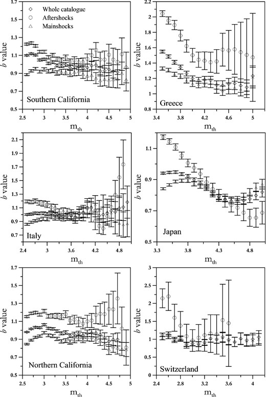
The b values as a function of mth for main shocks, aftershocks and whole catalogues after declustering with the Felzer & Brodsky (2006) algorithm. The legend in the SC panel is valid for the other catalogues.
We explicitly test this hypothesis by means of simulations of the ETAS model (Vere-Jones 1970; Ogata 1988, 1998; Kagan 1991). We generate 103 synthetic catalogues following the procedure described by Zhuang et al. (2004) and we implement a magnitude distribution with bm = 0.5 for main shocks and ba = 1.2 for aftershocks. These values have been chosen in order to obtain the best fit of the stacked experimental curve (Fig. 2). Magnitudes are in the range [3.5, mu]. The average b values well agree with the experimental ones for the cumulated catalogues when mu = 7. For larger values of mu, mm increase monotonically and the b increase (regime 3) becomes less pronounced. Numerical results confirm that the increase of b observed for some experimental catalogues could be interpreted as a finite size effect corresponding to the largest fault monitored in each catalogue. As a final remark we notice that simulations of the ETAS model with a constant b (bm = ba = 1.1∀m) and a sufficiently large mu = 9.5 provide a constant b(mth) (Fig. 2).
4 CONCLUSIONS
The analysis of the b value as a function of mth, performed for six earthquake catalogues, shows that the catalogues exhibit a continuous decrease of b for mth > mc (regime 2) followed by a subsequent increase (regime 3). This observation can be modelled assuming that b varies continuously with m. We have shown that the decrease of b with m can be related to the distribution of b. We have found that both a peaked continuous distribution and a binomial distribution provide a good representation of the experimental observations.
The continuous peaked distribution, that is usually not very different from a Gaussian distribution, could originate from the spatial and/or temporal variations of the b value. The binomial distribution, conversely, can be caused by different GR laws for main shocks and aftershocks. Within this scenario, the spatial and/or temporal variability of b, experimentally observed, can be attributed to the different ratio between the number of aftershocks and main shocks in different spatio-temporal regions. A declustering procedure seems to confirm this hypothesis, although the result could be a spurious effect: Generally declustering methods tends to consider large events as mainshocks and small events as aftershocks. We have explicitly shown that numerical simulations of ETAS catalogues, where main shocks and aftershocks are distributed with different b values, reproduce the behaviour experimentally observed. Numerical simulations also provide an explanation for the increases of b(m) for large magnitudes that can be attributed to an upper magnitude cut-off in experimental catalogues.
In alternative to the above interpretations, the b dependence on mth could also be an artefact due to instrumental and technical problems in the evaluation of earthquake magnitudes. Within this hypothesis our non-linear fit represents the best way to correct experimental magnitudes
Our results have strong implications in seismic hazard evaluation. Indeed a smaller b value for main shocks increases significantly the probability for large events in seismogenic areas with important consequences for the seismic risk evaluation. Conversely, the presence of a large magnitude cut-off in the GR distribution introduces a finite size effect that decreases the expected rate. Both effects should be taken into account and eventually investigated in other geographic regions.
