Article

A Year-Round Measurement of Water-Soluble Trace and Rare Earth Elements in Arctic Aerosol: Possible Inorganic Tracers of Specific Events

1
Institute of Polar Sciences, National Research Council of Italy (ISP-CNR), 30172 Venice, Italy
2
Department of Environmental Sciences, Informatic and Statistics, University Ca’ Foscari, 30172 Venice, Italy
*
Author to whom correspondence should be addressed.
Atmosphere 2021, 12(6), 694; https://doi.org/10.3390/atmos12060694
Submission received: 23 April 2021 / Revised: 24 May 2021 / Accepted: 27 May 2021 / Published: 29 May 2021
(This article belongs to the Special Issue Air Pollution in the Polar Regions: Levels, Sources and Trends)

Abstract

:
This study presents the year-round variability of the water-soluble fraction of trace elements (wsTE) and rare earth elements (wsREE) among size segregated airborne particulate matter samples collected at Ny-Ålesund in the Svalbard Archipelago from 26 February 2018 to 26 February 2019. Six different aerosol dimensional fractions were collected using a multi-stage Andersen impactor to better understand local and global circulation with the aim of disentangling the source of inorganic tracers from specific natural or anthropogenic sources. The wsTE and wsREE content, especially in the finest fractions in remote areas, is primarily related to long-range transport and it gives valuable information on (1) the global circulation, (2) the natural sources and (3) the contribution of human activities to aerosol composition. A Factor Analysis was applied to the dataset, including levoglucosan and methanesulfonic acid (MSA), to assess the possibility of using certain inorganic tracers as indicators of specific transport events or circulation regimes. We also investigate back-trajectories to determine potential source areas.

1. Introduction

Polar regions are widely acknowledged as important areas for studying the effect of climate change, the impact of anomaly natural events and human activities on the climate itself. Warming in the Arctic has occurred much more rapidly than the global average and in particular the Ny-Ålesund archipelago has experienced a significant rise in temperature over the last two decades [1]; this phenomenon is known as Arctic amplification [2].
Particulate matter can influence the chemical and radiative properties of the atmosphere. These particles can transport material through the atmosphere, and they can act as cloud condensation nuclei (CCN), affecting the optical properties of the atmosphere [3]. The transport of particulate matter (PM) from low and medium latitudes towards the polar regions may dramatically impact the quality of these fragile areas. To understand the role that aerosol could have in variation in the budget of solar radiation, reduction of visibility and possible pollution of the ecosystem [4,5], it is useful to know the geochemical characteristics of the PM that reach Arctic areas. In addition, the aerosol composition could significantly affect the snow pack chemical composition and the load of specific elements [6]. Another important property of the aerosols is their size distribution, giving valuable information on the sources of these aerosols and on the atmospheric processes modifying their properties during atmospheric transportation.
The investigation of the chemical composition of Arctic aerosol is essential to discriminate between local sources or long-range atmospheric transport processes in order to define also the impact of the deposition of this material on the Arctic snowpack. The last 10 years’ studies reported in the literature on Arctic aerosols focused on major ions [7,8], methansulfonic acid (MSA) [9], anhydrosugars [10,11], amino acids [12,13,14], black carbon (BC) [15,16] and also secondary organic aerosol (SOA) [17]. Despite their low concentrations, trace elements (TE) and rare earth elements (REE) are important components of aerosol. These elements already have been investigated in Arctic aerosols [18], but these studies are often limited to some seasons. A multiyear investigation about TE concentrations was conducted during four successive spring–summer sampling campaigns (2010–2013) at Ny-Ålesund [19]. Some studies were performed regarding the REE concentration in aerosol collected in remote sites [18,20,21], but the knowledge about these species are limited due to the analytical limitations to obtain limits at ultra-trace concentrations.
Transported to polar regions, they may provide important information about local and global circulation and on source areas principally due to conservative behaviour of certain elements like REE and some TE when transported by aerosol. In winter and spring, the air masses efficiently reach the Arctic areas from mid latitudes, in particular from Eurasia, while in summer and autumn the circulation is reduced due to a weaker vertical stratification [16,17,19,22]. Elements deriving from various sources, such as volcanic emissions, biomass burning and anthropogenic activities, such as agricultural fires, are generally related to the finest component of aerosol and having a long residence time in the atmosphere can be the result of a long transport [20,23,24].
In this paper, we present the results of an analysis of the six dimensional fractions of 46 samples collected during a one-year sampling campaign that took place from 26 February 2018 to 26 February 2019 at Ny-Ålesund in the Svalbard Archipelago (Figure S1), with a time resolution from 6 to 10 days. We will evaluate the seasonal variation in Arctic aerosol of 27 TE (Li, Be, Mg, K, Ca, V, Cr, Mn, Fe, Co, Ni, Cu, Zn, Ga, As, Y, Rb, Sr, Ag, Cd, Cs, Ba, Tl, Pb, Bi, U and Th) and 14 REE (La, Ce, Pr, Nd, Sm, Eu, Gd, Tb, Dy, Ho, Er, Tm, Yb and Lu). We chose to assess the water-soluble fraction to directly compare the inorganic fraction with the corresponding organic fraction [17], and whether or not this inorganic component will be able to recognize specific events as the organic component does. In addition, using a multi-stage impactor, we will also attempt to differentiate short-term versus long-term inputs to evaluate what has the most impact over the course of a year. As described in Feltracco et al. (2021) [17], a multi-stage impactor was used to sampling aerosol in six dimensional fractions to better evaluate and differentiate local and long-range inputs. This is the first investigation about the annual trend in the size segregated TEs and REEs in Arctic aerosol.

2. Materials and Methods

2.1. Sampling

Forty-six aerosol samples were collected from 26 February 2018 to 26 February 2019 in the Gruvebadet atmospheric laboratory (Svalbard Islands, 78°55′03″ N, 11°53′39″ E, 50 m a.s.l.), close to Ny-Ålesund and 1.4 km far from the Kongsfjorden.
As described in Feltracco et al. (2021) [17], a multi-stage Andersen impactor (TE-6000 series, Tisch Environmental Inc., Cleves, OH, USA) was used to collect aerosol samples on six pre-combusted (4 h at 400 °C in a muffle furnace) quartz fibre filters. The sampler accumulated particles with cut-off diameters of 10.0 μm, 7.2 μm, 3.0 μm, 1.5 μm and 0.95 μm on slotted quartz fibre filters (QFF) and <0.49 μm on the backup filters (also reported in this paper as “stages” and “dimensional fractions”). The frequency of sampling was 6 days in spring and summer and 10 days in autumn and winter, following the results and the protocols of previous campaigns [11,18]. The mean total air volume was 9000 and 16,000 m3, respectively. The details about the collection period are reported in Table S1. Field blanks were obtained using filters installed on the sampler for 5 min with the air pump switched off. Samples and blanks were stored at −20 °C until analysis. Referring to the division in seasons, we adopted the following intervals: end-Winter 2018, from 26 February 2018 to 27 March 2018; Spring 2018, from 27 March 2018 to 25 June 2018; Summer 2018, from 25 June 2018 to 25 August 2018; Autumn 2018, from 3 October 2018 to 24 December 2018; and Winter 2018–2019, from 24 December 2018 to 26 February 2019.

2.2. Instrumental Analysis

The description of the sample treatment has been reported in five previous studies [10,13,14,17,18]. Briefly, the slotted and backup QFF were cut in half using stainless-steel scissors that were previously washed with methanol. Each filter was extracted twice in an ultra-sonic bath at 10 °C for 15 min using ultrapure water. The slotted filters and the back-up filters were extracted in a first step with 9 and 25 mL of ultrapure water followed by a second step with 1 and 5 mL of ultrapure water, respectively. The extracts were unified, filtered, using a 0.45 µm polytetrafluoroethylene (PTFE) filter (Whatman, Maidstone, Kent, UK), and immediately frozen until the analysis. All samples and field blank filters were handled inside an ISO5 clean room under a laminar flow bench (class 100) to avoid any contamination from laboratory air particles.
All 300 samples (46 collected samples per 6 fractions plus 4 blanks per 6 fractions) were analysed at the Institute of Polar Sciences-CNR/University of Ca’ Foscari laboratories in Venice to determine TE and REE by means of an iCAP-RQ ICP-MS (Thermo Scientific™, Bremen, Germany) equipped with an autosampler. Analyses were performed on acidified samples (2% v/v of ultrapure nitric acid, Romil™ UPA, Cambridge, UK) and quantification was done using the external calibration method. The multi-elemental stock solutions used for TE and REE were IMS102 and IMS101 by Ultra Scientific (Santa Clara, CA, USA), respectively. Standards at concentrations of 0, 10, 20, 50, 100, 200 and 500 ng·L−1 and 1, 5, 10, 50 and 100 µg L−1 for TE and 0, 2, 5, 10, 20, 50, 100 and 200 ng·L−1 for REE were prepared gravimetrically, adding the appropriate quantity of a multi-elemental stock solution (IMS102 and IMS101 by Ultra Scientific, respectively). During each session of analysis, also six blank solutions were repeatedly analysed to evaluate the detection limits, calculated as three times the standard deviation of six blanks.
Levoglucosan and methanesulfonate (MSA) were used as specific markers for biomass burning and phytoplankton blooms, in comparison with the concentration of wsTE and wsREE to confirm potential emission sources. The determination and quantification of these compounds were already described elsewhere [25]. We used an ion chromatograph (Thermo Scientific™ Dionex™ ICS-5000, Waltham, MA, USA) coupled with a single quadrupole mass spectrometer (MSQ Plus™, Thermo Scientific™, Bremen, Germany). Briefly, the determination of levoglucosan was performed using a CarboPac MA1™ analytical column (Thermo Scientific, 2 × 250 mm) equipped with an AminoTrap column (2 × 50 mm). The NaOH eluent gradient at a flow rate of 0.25 mL min−1 was as follows: 20 mM (0–23 min), 100 mM (23–43 min) and 20 mM (43–53 min). The injection volume = 50 µL. Quantification was performed using labelled 13C6-levoglucosan as the internal standard. MSA determination was achieved using an anionic exchange column (Dionex Ion Pac AS11 2 × 250 mm) and a guard column (Dionex Ion Pac AG11 2 × 50 mm). The NaOH gradient at a flow rate of 0.25 mL min−1 was as follows: 0–3.5 min gradient from 0.5 to 5 mM; 3.5–5 min gradient from 5 to 10 mM; 5–25 min gradient from 10 to 38 mM; 25–30 min, column cleaning with 38 mM; 30–35 min; and equilibration at 0.5 mM. The injection volume = 100 µL. Quantification was achieved using an external calibration curve. All specific details about the instrumental and methodological parameters are reported in previous papers [10,26].

2.3. Enrichment Factor

The use of trace element enrichment factors (EFs) relative to the Earth’s crust concentrations is useful in highlighting the contribution of non-natural sources to elemental levels. EF is calculated as follows:
EF i = ( i j ) a t m o s p h e r e ( i j ) u p p e r   c r u s t
where EFi is the enrichment factor of element i, j is a reference element of crustal origin, (i/j)atmosphere is the ratio of element i to element j in the atmosphere and (i/j)upper crust is the ratio of element i to element j in the upper crust. The composition of the upper crust was described in Wedepohl et al. (1995) [27] while, following the suggestion of Gao et al. (1992) [28], we used Al as the reference element in the EF calculations. An EF near 1 indicates a crustal derived element (geogenic), while significantly higher EF values indicate a non-crustal-derived element (non-geogenic): an EF between 10 and 100 indicates a moderate enrichment while an EF above 100 indicates a prevalent non-crustal origin. Calculating the EFs allows us to make a starting estimate of the potential source of various elements but the indications obtained must be confirmed by other evaluations.
To estimate the influence of marine source we also calculated the marine EFs (MEFs) relative to sea water concentrations, using the abundance in sea water reported by Nozaki et al. (2010) [29]. MEFs were calculated as
MEF i = ( i j ) a t m o s p h e r e ( i j ) s e a   w a t e r
Mg was used as a reference element (j) of marine origin. Analogous to the EF, an MEF near 1 indicates a marine-derived element, while higher values indicate moderate (10–100) to high (>100) enrichment relative to sea water.

2.4. Chemometric Approach and Back Trajectories Analysis
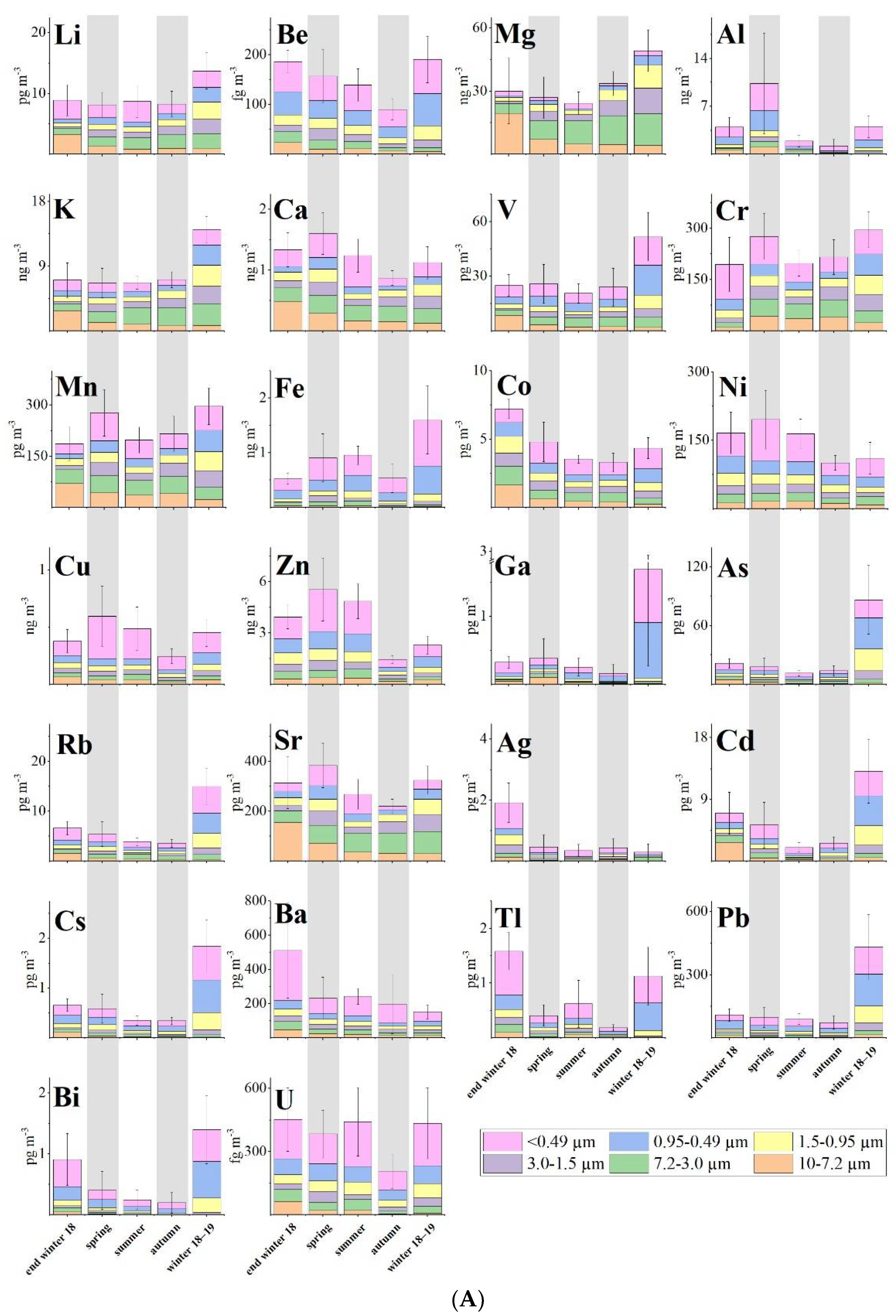
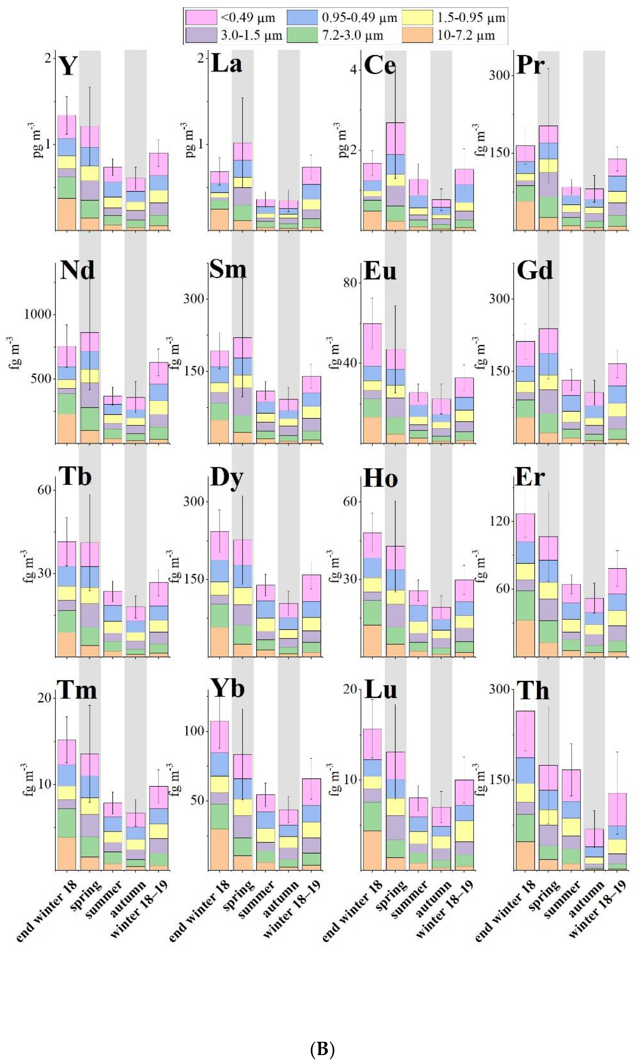
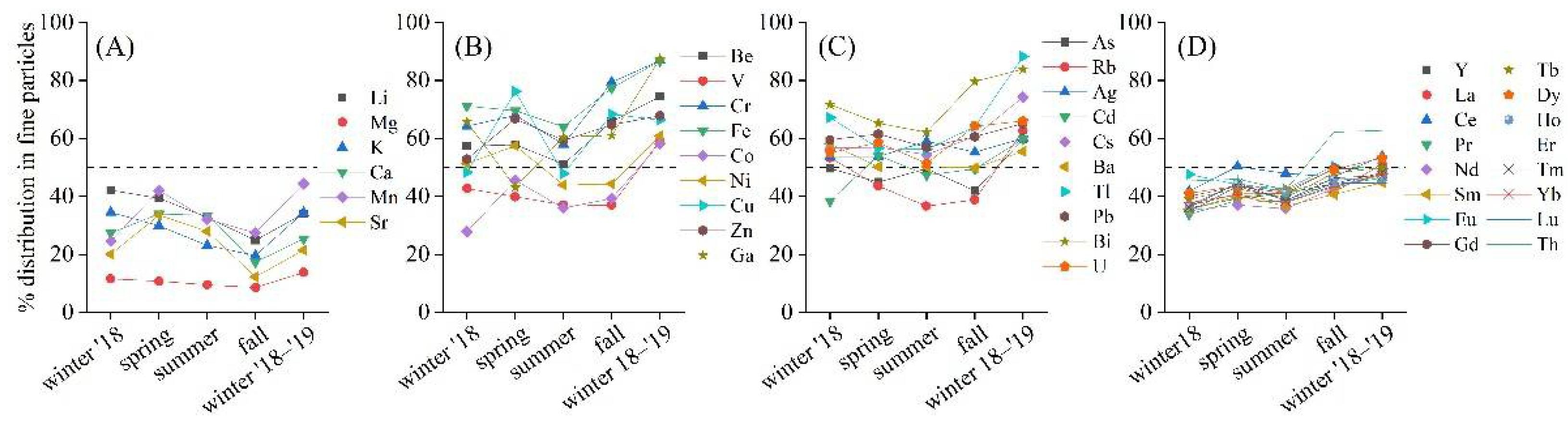
Factor Analysis (FA) is a chemometric approach that allows us to reduce the size of our data matrix without losing the information it contains. FA with varimax rotation was performed on the auto-scaled data matrix using Statistica 10.0 (StatSoft, Inc., 2011, Hamburg, Germany) [30]. The varimax rotation is the most commonly rotation strategy used with the aim to better clarify the pattern of loading, highlighting the variables that mark the extracted factors. The concentrations below the method detection limit (MDL) were substituted with a value of ½ MDL in the FA. Data are presented as a plot of two factors; the X,Y values for each sample represent the importance of the variables that characterize the factor, for that sample itself, giving an estimation if the sample is related to a certain factor or not. High values of a factor indicate its importance for the sample.
To understand the general transport pattern of air masses recorded at the sampling site, backward air trajectories ending at the Gruvebadet aerosol laboratory were computed using Hybrid Single-Particle Lagrangian Integrated Trajectories (HYSPLIT) transport and dispersion models [31,32]. Back trajectories were calculated using a vertical velocity model with an endpoint at 500 m above ground level and starting a trajectory every 6 h. Knowing that airborne particles in the troposphere have typical lifetimes of 3–10 days on average, also considering dry and wet deposition, we chose to compute 7-days back trajectories [33]. The meteorological data used for computing all the backward trajectories were the NCEP/GDAS (Global Data Assimilation System) at a 1 × 1° resolution. Based on the backward particle release simulation, the cluster aggregation was displayed for each month (Figure S2).

3. Results

All six dimensional fractions of each sample collected during the February 2018 to February 2019 campaign were analysed to determine the content of the water-soluble REE (La-Lu) and water-soluble TE (Li, Be, Mg, K, Ca, V, Cr, Mn, Fe, Co, Ni, Cu, Zn, Ga, As, Y, Rb, Sr, Ag, Cd, Cs, Ba, Tl, Pb, Bi, U, Th) content (Figure 1A,B). The concentrations of wsTE and wsREE determined in the PM10 samples are shown in Supplementary Tables S2 and S3. All reported values are blank-corrected. Mg (30 ± 13 ng m−3), K (5 ± 2 ng m−3), Zn (3 ± 2 ng m−3), Ca (1.1 ± 0.4 ng m−3) and Fe (0.8 ± 0.2 ng m−3) were the most concentrated wsTE in the whole sampling period, considering PM10 (as the sum of all stages). The other wsTE were abundantly <1 ng m−3. Mg, K, Ca, Li and Mn were mainly distributed above 0.95 µm (coarse fraction), suggesting a local source (Figure 1A and Figure 2A). These metals did not show a valuable shift in the particle-size distribution during the whole sampling period, while the other wsTE varied remarkably among the season with a shift in the fine fraction in spring and in winter (Figure 1A and Figure 2B,C).
The most abundant wsREE was Ce (2 ± 1 pg m−3), followed by La (0.6 ± 0.5 pg m−3) and Nd (0.6 ± 0.4 pg m−3), following the normal order of abundance of most crustal materials (Ce > La > Nd > Sm > Yb). The wsREE were equally distributed between coarse and fine fractions (Figure 1B). A slight shift toward the fine fraction in winter was detected (Figure 2D).
The concentrations found in this campaign were comparable with the PM10 values determined during spring and summer in some previous studies at Gruvebadet laboratory [2,9,34] and in the Chinese Arctic “Yellow River Station” at Ny-Ålesund [35].
The shift reported toward the fine fraction in spring and winter is frequently linked with an increase in concentration of wsTE and wsREE (Figure 2). This suggest that the long-range atmospheric transport (LRAT) seems to be the dominant factor of the presence of metals in the Arctic atmosphere.

4. Discussion

The year-round study of chemical composition of PM particle-size distribution, gathered from February 2018 to February 2019 at Ny-Ålesund, a key region to understand air mass circulation, provides new information about the origin of the PM and the importance of their different dimensional size in discriminating possible source areas and specific events. The back-trajectory evaluation helps us to interpret the results (Figure S2) because this method is widely used in recognizing the routes of pollutants [36]. In fact, the back trajectories distinctly indicate that the source areas were strictly related to seasonality. During summer, transport from the mid-latitudes decreased due to the contraction of the polar vortex, while in winter the long-range atmospheric transport covers a more extended area [23].
Different approaches were applied to interpret the results and to recognize the PM sources using wsTE and wsREE as tracers. Firstly, we considered the EFs calculated for all analysed elements related both to the upper crust and seawater composition. Then, the geogenic or non-geogenic origin of the samples was evaluated using ternary diagrams applied to REEs. Finally, a chemometric approach was used to reduce the number of variables and to link the inorganic and organic components of samples. In fact, Factor Analysis (FA) was performed, including in our dataset also levoglucosan and MSA. Levoglucosan is recognized as a tracer of biomass burning [37] while MSA is related to algal bloom [38], suggesting primary marine production as the source.

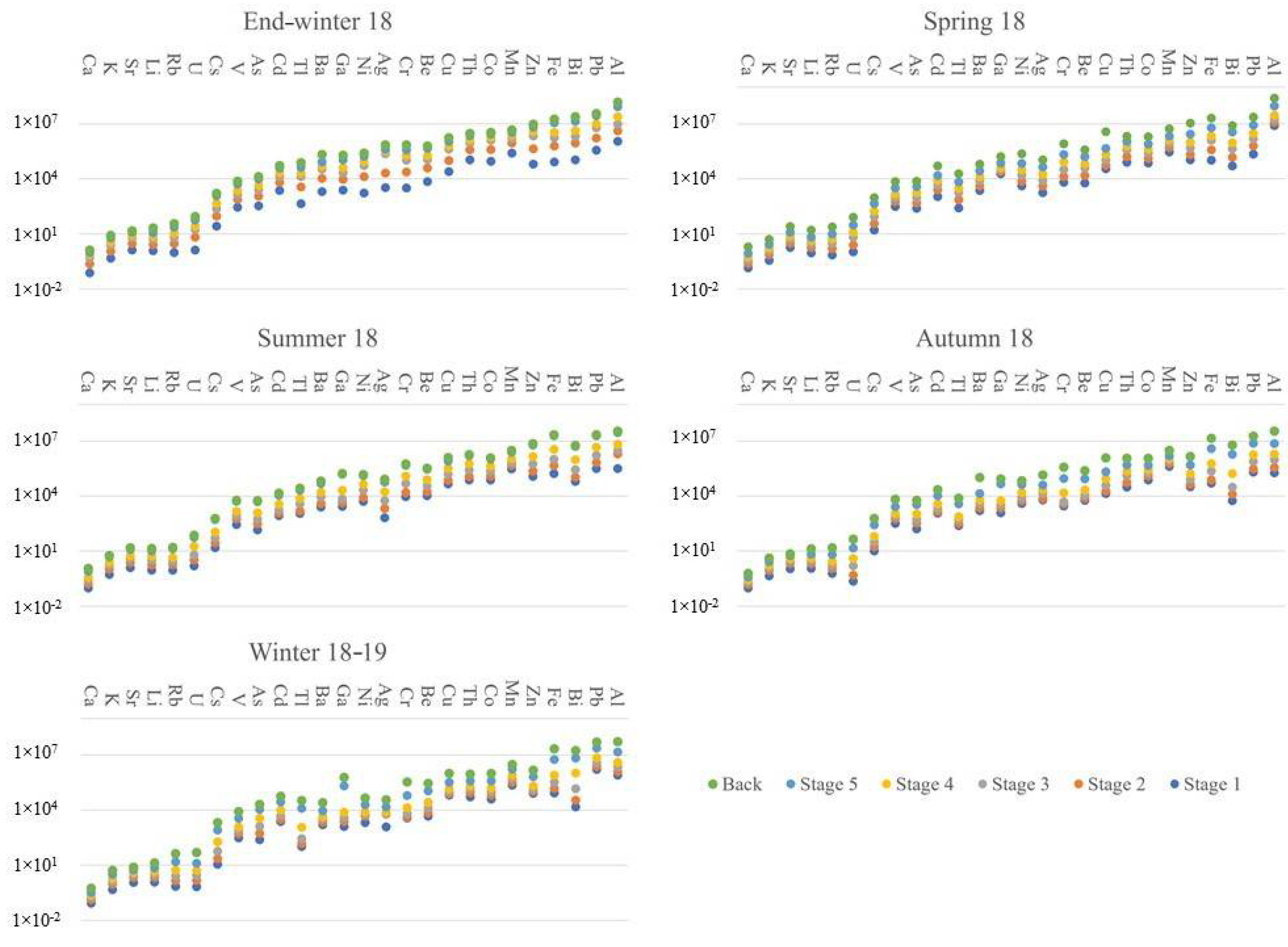
4.1. Enrichment Factors

The Figure 3 shows the EFs calculated for the measured TE from end-winter 2018 to winter 2019 as an average of the seasonal trend related to the upper crust composition [27]. Zn, Cd, Cu and As are the most enriched elements with values above 100, indicating a non-geogenic origin. Ag, Pb, Ni, Cr and Bi have values around 100, indicating that they are only weakly related to the crust. Th, Fe, Ga, REE, Rb, Ca, Be, Cs, Y and U, with values quite always below 10, show a geogenic origin. K, V, Li, Mn, Ba, Co, Tl, Sr and Mg have values that indicated a probably geogenic source; but, especially in Summer and Fall, these elements have values around 100 or higher, indicating probable mixed sources. Values strongly above 100 from Bi, Cr, Ni, Pb, Ag, As, Cu, Cd and Zn suggest that anthropogenic sources are responsible for the concentrations of these elements. These values are according to the previous results reported by Turetta et al. (2016) [18], where the investigation of the particle-size distribution of these species was performed.
It has to be noted that, during summer, the EF values of all stages are similar for each wsTE due to the presence of local sources as the main input. In contrast, during winters and spring, different values of EFs are found in the different stages because long-range transport plays an important role in the PM composition. Although size distribution is not directly correlated to EFs, the information about the EF values in the different stages can support the seasonal variation of input in the Arctic atmosphere.
The MEFs (Figure S3A,B) were calculated for all elements analysed as an average of the seasonal trend related to the seawater mean composition [29]. Ca and K have values close to 1, confirming their marine origin. Li, with values between 1 and 10, Rb, with values between 1 and 30, and U, with values between 2 and 50, seem to have a prevailing marine input but other sources must be considered. Figure S3B emphasizes the differences between seasons, highlighting the importance of the dimensional size of the elements of mixed origin. In spring, a higher variability is observed for those sizes with a possible long-range origin, while in summer the finer fractions do not seem to be relevant. End-winter 2018 and Winter 2019 seems to be quite different, but it is to note that both seasons show the same trend of considered marine origin elements and a relevant contribution of long-range transport for those elements of mixed origin. All other elements, with values higher than 100, appear to have sources other than the marine one. From the comparison between the two calculated series of EFs, related to the Upper Crust and Sea Water composition, respectively, we can hypothesize that the mixed source detected by the EFs for Ca, K, Sr, Li, Rb and U could be related to marine inputs due to the fact that their MEF values range between 1 and 50.

4.2. Ternary Diagrams

With the aim to understand the potential sources of the analysed elements, we evaluate our data using ternary diagrams applied to REEs to evaluate the geogenic or non-geogenic origin of the samples. The diagram in Figure 4a compares La–Ce–Sm, whose values were adjusted to put the crustal concentration in the center of the ternary plot. The coarse fraction (10–3 µm) is prevailingly distributed around the crustal position while the medium fraction (3–0.95 µm) shows a displacement from the crustal composition towards lower values of Ce and higher values of Sm. Finally, the fine fraction (<0.95 µm) highlights a displacement of samples towards higher values of Ce and lower values of La and Sm. Dispersion of samples away from the upper crust composition indicates a likely anthropogenic influence on REE composition, particularly in the medium and fine fractions.
In Figure 4b, we report the ternary diagram V–Ce–La to highlight the anthropogenic sources that can characterize our samples. It is known from the literature that V can help distinguish different potential anthropogenic sources when compared with some REEs. In particular, V may differentiate the contributions of emissions from ships or other oil combustion processes from those of refineries or motor vehicles [19,39,40].
Our samples are principally in the right corner, the V apex, indicating as prevailing source the oil combustion, but it is to note that the position of a relevant part of samples shifts from the V apex toward the crustal composition, especially samples of medium and fine dimensions. This shift could indicate a mixed source for these samples: oil combustion and weathering of the surface are the more probable, but, due to a displacement toward high values of Ce of some samples, we cannot exclude motor vehicles as a possible source.
V and Ni can be also used as typical markers for fossil fuel combustion from ships. Viana et al. (2008) [40] established V and Ni as valid tracers of shipping emissions, with a typical V/Ni ratio of 2.5–3.0. In order to better characterize this factor, the V/Ni ratio was calculated: the ratio was always below 1 during the whole sampling period. Furthermore, V and Ni showed only a slight concentration increase during the 20–25 June and 14–19 July samples (215 and 186 pg m−3, respectively). The wind roses in the first period (Figure S4) suggest a source of the particles from the fjord due to ship emissions. On the contrary, from 13 to 19 June, no favourable winds were detected. Considering that the marine traffic in the Kongsfjorden is generally high in June and July (3 to 10 landing ships per day in the Ny-Ålesund harbour), no valuable relation between local ship emission and V and Ni was reported in 2018.

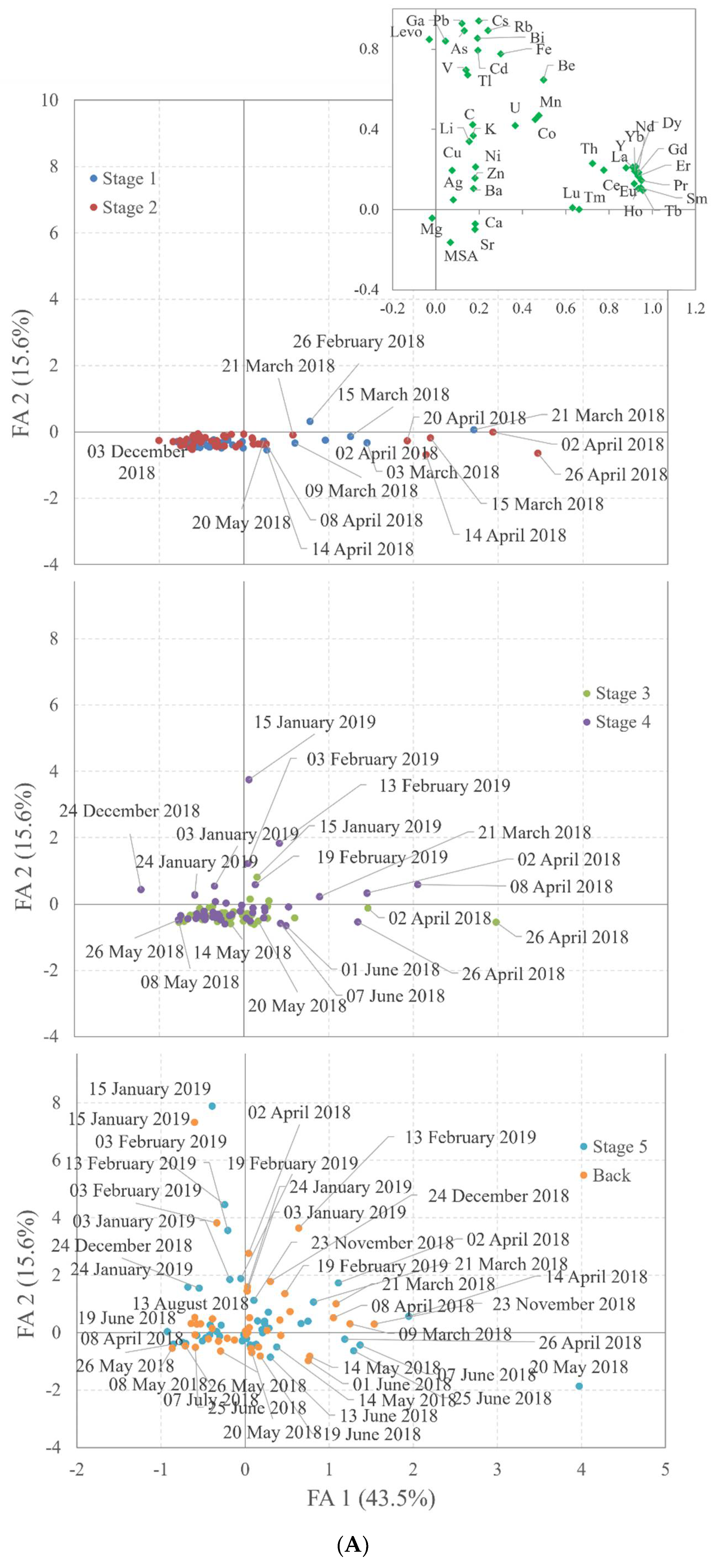
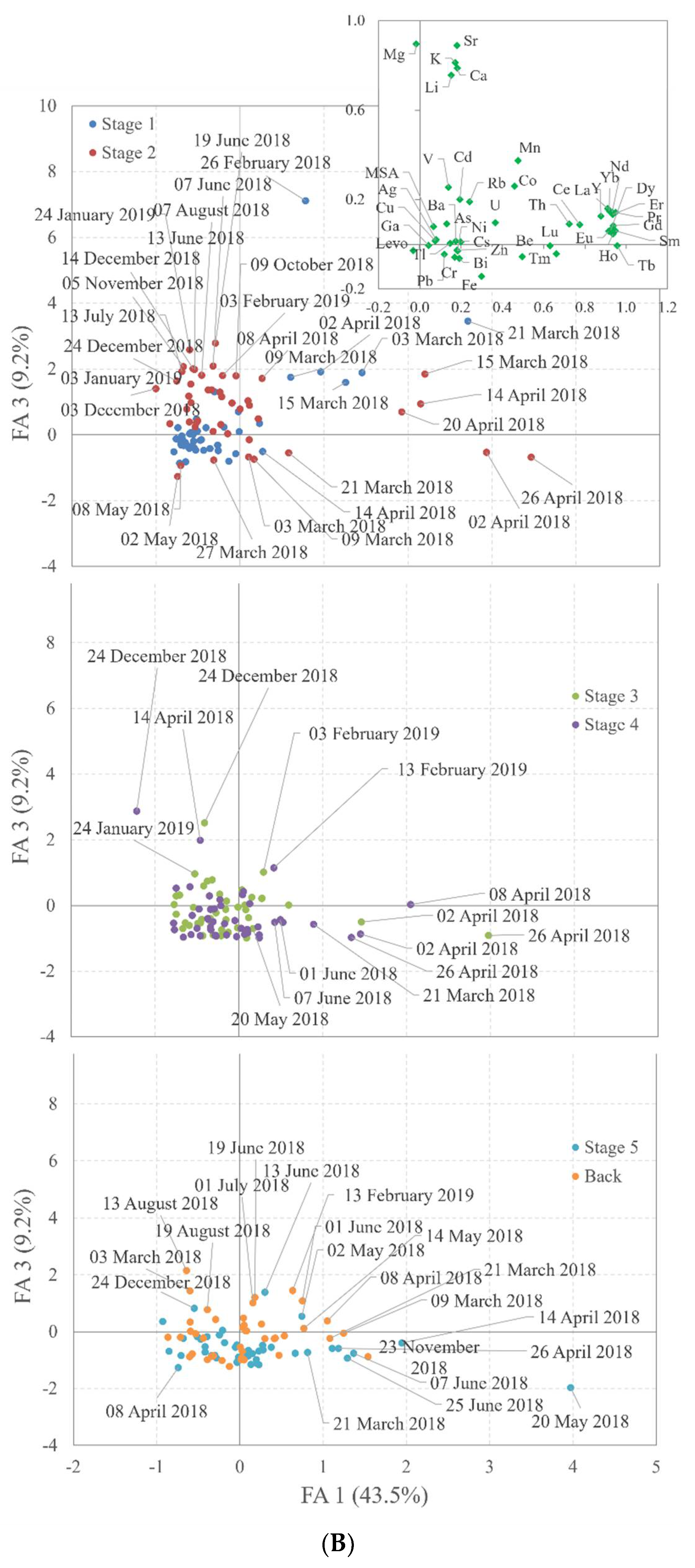
4.3. Chemometric Evaluation

With the aim to better evaluate all samples and all variables together, and considering the dimension of our data-matrix, 276 samples (46 samples per 6 dimensional fractions) per 41 elements plus 2 organic compounds used to compare inorganic results with the information obtained from organic fraction, we have performed a statistical evaluation of all the data. In particular, Factor Analysis was performed, extracting four factors that account together for 75.6% of the explained variance.
In Figure 5 and Figure S5, we present the results of the FA as graphs of all the samples subdivided for the dimensional fractions in order to highlight the differences between the dimensions with respect to the possible sources. For clarity, we have plotted in three separate graphs the results obtained from the FA for each couple of factors on a dimensional basis. The particle-size distribution influences the results of the FA because the difference between wsTEs and wsREEs is clearly shown in Table 1, where the wsREEs are loaded in Factor 1.
The four extracted factors (Table 1) account together for 75.6% of the explained variance. The first factor brings together all REEs and Be, Mn, Co and U; the second levoglucosan, Be, V, Fe, Ga, As, Rb, Cd, Cs, Tl, Pb and Bi; the third Li, Mg, K, Ca and Sr; and the fourth MSA, Cr, Ni, Cu and Zn. Considering these clusters of elements, we can hypothesize Factor 1 (F1) as related to crustal source. In the score plot (Figure 5A), on the basis of F1, the separation of the samples collected in spring, from March to April in coarser fractions and from March to June for finer ones, is evident compared to the others. This separation could be related to meteorological factors considering that springtime is very often characterized by strong winds. Factor 2 (F2) seems to be related to combustion, both biomass burning, as suggested from the presence in this factor of levoglucosan, and oil combustion, as suggested from V. In the finer fractions, this factor separates winter samples from all the others, while no-separation is evident in coarser fractions. The seasonal variation, showing elevated concentrations in winter (Tables S2 and S3), may be due to the transport from the midlatitudes to the Arctic intensifying during the winter and spring [22,23,41], as confirmed also by the back trajectories (Figure S2) that well overlay the Northern Russian areas. Factor 3 (F3), mainly associated with elements related to marine origin, seems partially separate, both in the finer and coarser fractions, in the spring–summer samples compared to the others, with some exceptions, such as the sample from 26 February 2018 that show a high value for F3 (Figure 5B). The importance of the marine source in the summer samples is related to the lack of sea-ice cover and to the input from the Arctic Ocean in those periods, as highlighted from back trajectory evaluations (Figure S2). The medium fractions seem to be not affected by this factor. Factor 4 (F4), related to marine primary production on the basis of the presence of MSA, seems to have a strong effect only on the finest fraction (<0.49 µm), separating the summer and partially spring samples from the others (Figure S5). The presence of micronutrients, such as Cu and Zn, support this interpretation of F4.

5. Conclusions

On the basis of all the presented data, we can conclude that the year-round sampling campaign lets us evaluate the evolution of PM through the different seasons in an Arctic area and gives an indication of the possible source areas for PM that reach the Arctic. In particular, the one-year sampling allowed us to recognize the different sources that contribute to the composition of wsTE and wsREE in particulate matter: crust source, combustion, marine inputs and marine primary productivity. On the other hand, the six different dimensional sizes of the samples separate, in the same season, the short-range from long-range contributions, highlighting the crustal source and different anthropogenic sources; for example, ternary diagrams help us to recognize both vehicular traffic and oil combustion inputs. The information obtained considering EFs, ternary diagrams and Factor Analysis, with the support of back-trajectory analyses, confirms the ability of TE and REE in tracing PM, both in terms of source area and seasonality when different dimensional sizes of the particles are considered.
From the comparison with previous research, in the same area, we can state that one year is probably not enough to fully understand the behaviour of TEs and REEs. However, this comparison makes it possible to hypothesize a similar behaviour for the same season in different years, obviously considering the ever-possible local variability and the occurrence of specific events, such as a volcanic eruption or wildfires.
The importance of recognizing sources of PM is highlighted here: the pollutants and, more generally, PM reaching the Arctic regions from the mid-latitudes may result in potential negative feedback regarding climate change. To understand if and how the PM is related to short- or long-range transport, and to different dimensional sizes, can help us in recognizing the role that it plays in the Earth’s climate system.

Supplementary Materials

The following are available online at https://www.mdpi.com/article/10.3390/atmos12060694/s1. Ref. [42] cited in Supplementary Table S1.

Author Contributions

Conceptualization, C.T., M.F. and E.B.; methodology, C.T. and M.F.; software, C.T., M.F. and E.B.; validation, C.T. and M.F.; formal analysis, C.T. and M.F.; investigation, C.T., M.F. and E.B.; resources, C.T. and A.G.; data curation, C.T., M.F. and E.B.; writing—original draft preparation, C.T., M.F. and E.B.; writing—review and editing, C.T., M.F. and E.B.; visualization, C.T., M.F. and E.B.; supervision, A.S., A.G. and C.B.; project administration, A.G.; funding acquisition, A.G. All authors have read and agreed to the published version of the manuscript.

Funding

This research received no external funding.

Institutional Review Board Statement

Not applicable.

Informed Consent Statement

Not applicable.

Data Availability Statement

Some data reported in this study are available here: https://doi.org/10.1594/PANGAEA.928238 [43].

Acknowledgments

This study is a result of the multi and interdisciplinary research activities based at the Arctic Station Dirigibile Italia, managed and coordinated by the Institute of Polar Sciences of the National Research Council of Italy. We acknowledge the help of ELGA LabWater in providing the PURELAB Pulse and PURELAB Flex, which produced the ultrapure water used in these experiments. The authors gratefully acknowledge the NOAA Air Resources Laboratory (ARL) for the provision of the HYSPLIT transport and dispersion model and READY website (http://www.ready.noaa.gov (accessed on 25 May 2021)) used in this publication.

Conflicts of Interest

The authors declare no conflict of interest.

References

  1. Maturilli, M.; Hanssen-Bauer, I.; Neuber, R.; Rex, M.; Edvardsen, K. The Atmosphere Above Ny-Ålesund: Climate and Global Warming, Ozone and Surface UV Radiation. In The Ecosystem of Kongsfjorden, Svalbard; Springer: Cham, Switzerland, 2019; pp. 23–46. ISBN 978-3-319-46425-1. [Google Scholar]
  2. Serreze, M.C.; Barry, R.G. Processes and impacts of Arctic amplification: A research synthesis. Glob. Planet. Chang. 2011, 77, 85–96. [Google Scholar] [CrossRef]
  3. Seinfeld, J.H.; Pandis, S.N. Atmospheric Chemistry and Physics: From Air Pollution to Climate Change; Wiley: New York, NY, USA, 2006; ISBN 9780471720171. [Google Scholar]
  4. Haywood, J.; Boucher, O. Estimates of the direct and indirect radiative forcing due to tropospheric aerosols: A review. Rev. Geophys. 2000, 38, 513–543. [Google Scholar] [CrossRef]
  5. Landsberger, S. Multielemental composition of the Arctic aerosol. JGR Atmos. 1990, 95, 3509–3515. [Google Scholar] [CrossRef]
  6. Spolaor, A.; Moroni, B.; Luks, B.; Nawrot, A.; Roman, M.; Larose, C.; Stachnik, Ł.; Bruschi, F.; Kozioł, K.; Pawlak, F.; et al. Investigation on the Sources and Impact of Trace Elements in the Annual Snowpack and the Firn in the Hansbreen (Southwest Spitsbergen). Front. Earth Sci. 2021, 8, 1–10. [Google Scholar] [CrossRef]
  7. Giardi, F.; Becagli, S.; Traversi, R.; Frosini, D.; Severi, M.; Caiazzo, L.; Ancillotti, C.; Cappelletti, D.; Moroni, B.; Grotti, M.; et al. Size distribution and ion composition of aerosol collected at Ny-Ålesund in the spring-summer field campaign 2013. Rend. Lincei 2016, 27, 47–58. [Google Scholar] [CrossRef] [Green Version]
  8. Udisti, R.; Bazzano, A.; Becagli, S.; Bolzacchini, E.; Caiazzo, L.; Cappelletti, D.; Ferrero, L.; Frosini, D.; Giardi, F.; Grotti, M.; et al. Sulfate source apportionment in the Ny-Ålesund (Svalbard Islands) Arctic aerosol. Rend. Lincei 2016, 27, 85–94. [Google Scholar] [CrossRef]
  9. Becagli, S.; Amore, A.; Caiazzo, L.; Di Iorio, T.; Sarra, A.; Lazzara, L.; Marchese, C.; Meloni, D.; Mori, G.; Muscari, G.; et al. Biogenic Aerosol in the Artic from Eight Years of MSA Data from Ny Ålesund (Svalbard Islands) and Thule (Greenland). Atmosphere 2019, 10, 349. [Google Scholar] [CrossRef] [Green Version]
  10. Feltracco, M.; Barbaro, E.; Tedeschi, S.; Spolaor, A.; Turetta, C.; Vecchiato, M.; Morabito, E.; Zangrando, R.; Barbante, C.; Gambaro, A. Interannual variability of sugars in Arctic aerosol: Biomass burning and biogenic inputs. Sci. Total Environ. 2020, 706, 136089. [Google Scholar] [CrossRef] [PubMed]
  11. Zangrando, R.; Barbaro, E.; Zennaro, P.; Rossi, S.; Kehrwald, N.M.; Gabrieli, J.; Barbante, C.; Gambaro, A. Molecular markers of biomass burning in Arctic aerosols. Environ. Sci. Technol. 2013, 47, 8565–8574. [Google Scholar] [CrossRef]
  12. Feltracco, M.; Barbaro, E.; Hoppe, C.J.M.; Wolf, K.K.E.; Spolaor, A.; Layton, R.; Keuschnig, C.; Barbante, C.; Gambaro, A.; Larose, C. Airborne bacteria and particulate chemistry capture phytoplankton bloom dynamics in an Arctic Fjord. Under Rev. Atmos. Environ. 2021, 256, 118458. [Google Scholar] [CrossRef]
  13. Feltracco, M.; Barbaro, E.; Kirchgeorg, T.; Spolaor, A.; Turetta, C.; Zangrando, R.; Barbante, C.; Gambaro, A. Free and combined L- and D-amino acids in Arctic aerosol. Chemosphere 2019, 220, 412–421. [Google Scholar] [CrossRef] [PubMed]
  14. Scalabrin, E.; Zangrando, R.; Barbaro, E.; Kehrwald, N.M.; Gabrieli, J.; Barbante, C.; Gambaro, A. Amino acids in Arctic aerosols. Atmos. Chem. Phys. 2012, 12, 10453–10463. [Google Scholar] [CrossRef] [Green Version]
  15. Stohl, A.; Berg, T.; Burkhart, J.F.; Fjæraa, A.M.; Forster, C.; Herber, A.; Hov, Ø.; Lunder, C.; McMillan, W.W.; Oltmans, S.; et al. Arctic smoke–record high air pollution levels in the European Arctic due to agricultural fires in Eastern Europe. Atmos. Chem. Phys. Discuss. 2006, 6, 9655–9722. [Google Scholar] [CrossRef] [Green Version]
  16. Eleftheriadis, K.; Vratolis, S.; Nyeki, S. Aerosol black carbon in the European Arctic: Measurements at Zeppelin station, Ny-Ålesund, Svalbard from 1998–2007. Geophys. Res. Lett. 2009, 36, 1–5. [Google Scholar] [CrossRef] [Green Version]
  17. Feltracco, M.; Barbaro, E.; Spolaor, A.; Vecchiato, M.; Callegaro, A.; Burgay, F.; Vardè, M.; Maffezzoli, N.; Dallo, F.; Scoto, F.; et al. Year-round measurements of size-segregated low molecular weight organic acids in Arctic aerosol. Sci. Total Environ. 2021, 763, 10. [Google Scholar] [CrossRef]
  18. Turetta, C.; Zangrando, R.; Barbaro, E.; Gabrieli, J.; Scalabrin, E.; Zennaro, P.; Gambaro, A.; Toscano, G.; Barbante, C. Water-soluble trace, rare earth elements and organic compounds in Arctic aerosol. Rend. Lincei 2016, 27, 95–103. [Google Scholar] [CrossRef]
  19. Conca, E.; Abollino, O.; Giacomino, A.; Buoso, S.; Traversi, R.; Becagli, S.; Grotti, M.; Malandrino, M. Source identification and temporal evolution of trace elements in PM10 collected near to Ny-Ålesund (Norwegian Arctic). Atmos. Environ. 2019, 203, 153–165. [Google Scholar] [CrossRef]
  20. Pacyna, J.M.; Ottar, B.; Tomza, U.; Maenhaut, W. Long-range transport of trace elements to Ny Ålesund, Spitsbergen. Atmos. Environ. 1985, 19, 857–865. [Google Scholar] [CrossRef]
  21. Giardi, F.; Traversi, R.; Becagli, S.; Severi, M.; Caiazzo, L.; Ancillotti, C.; Udisti, R. Determination of Rare Earth Elements in multi-year high-resolution Arctic aerosol record by double focusing Inductively Coupled Plasma Mass Spectrometry with desolvation nebulizer inlet system. Sci. Total Environ. 2018, 613–614, 1284–1294. [Google Scholar] [CrossRef]
  22. Quinn, P.K.; Shaw, G.; Andrews, E.; Dutton, E.G.; Ruoho-Airola, T.; Gong, S.L. Arctic haze: Current trends and knowledge gaps. Tellus Ser. B Chem. Phys. Meteorol. 2007, 59, 99–114. [Google Scholar] [CrossRef] [Green Version]
  23. Stohl, A. Characteristics of atmospheric transport into the Arctic troposphere. J. Geophys. Res. Atmos. 2006, 111, 1–17. [Google Scholar] [CrossRef]
  24. Toscano, G.; Gambaro, A.; Moret, I.; Capodaglio, G.; Turetta, C.; Cescon, P. Trace metals in aerosol at Terra Nova Bay, Antarctica. J. Environ. Monit. 2005, 7, 1275–1280. [Google Scholar] [CrossRef] [PubMed]
  25. Barbaro, E.; Kirchgeorg, T.; Zangrando, R.; Vecchiato, M.; Piazza, R.; Barbante, C.; Gambaro, A. Sugars in Antarctic aerosol. Atmos. Environ. 2015, 118, 135–144. [Google Scholar] [CrossRef]
  26. Barbaro, E.; Padoan, S.; Kirchgeorg, T.; Zangrando, R.; Toscano, G.; Barbante, C.; Gambaro, A. Particle size distribution of inorganic and organic ions in coastal and inland Antarctic aerosol. Environ. Sci. Pollut. Res. 2017, 24, 2724–2733. [Google Scholar] [CrossRef]
  27. Hans Wedepohl, K. The composition of the continental crust. Geochim. Cosmochim. Acta 1995, 59, 1217–1232. [Google Scholar] [CrossRef]
  28. Gao, Y.; Arimoto, R.; Duce, R.A.; Lee, D.S.; Zhou, M.Y. Input of atmospheric trace elements and mineral matter to the Yellow Sea during the spring of a low-dust year. J. Geophys. Res. 1992, 97, 3767–3777. [Google Scholar] [CrossRef]
  29. Nozaki, Y. Elemental Distribution: Overview; Turekian, K.K., Ed.; A derivative of Encyclopedia of Ocean Sciences; Academic Press: Cambridge, MA, USA, 2010; ISBN 9780080964836. [Google Scholar]
  30. Basilevsky, A. Statistical Factor Analysis and Related Methods: Theory and Application; John Wiley & Sons, Inc.: Hoboken, NJ, USA, 1994; ISBN 0471570826. [Google Scholar]
  31. Stein, A.F.; Draxler, R.R.; Rolph, G.D.; Stunder, B.J.B.; Cohen, M.D.; Ngan, F. Noaa’s hysplit atmospheric transport and dispersion modeling system. Bull. Am. Meteorol. Soc. 2015, 96, 2059–2077. [Google Scholar] [CrossRef]
  32. Draxler, R.R. An overview of the HYSPLIT_4 modelling system for trajectories, dispersion and deposition. Aust. Meteorol. Mag. 1998, 47, 295–308. [Google Scholar]
  33. Andreae, M.O. Aerosols before pollution. Science 2007, 315, 50–51. [Google Scholar] [CrossRef]
  34. Seinfeld, J.H.; Pandis, S.N. Atmospheric Chemistry and Physics: From Air Pollution to Global Change; Wiley: Hoboken, NJ, USA, 1998; Volume 1360. [Google Scholar]
  35. Zhan, J.; Gao, Y.; Li, W.; Chen, L.; Lin, H.; Lin, Q. Effects of ship emissions on summertime aerosols at Ny-Alesund in the Arctic. Atmos. Pollut. Res. 2014, 5, 500–510. [Google Scholar] [CrossRef] [Green Version]
  36. Stohl, A.; Forster, C.; Eckhardt, S.; Spichtinger, N.; Huntrieser, H.; Heland, J.; Schlager, H.; Wilhelm, S.; Arnold, F.; Cooper, O. A backward modeling study of intercontinental pollution transport using aircraft measurements. J. Geophys. Res. Atmos. 2003, 108. [Google Scholar] [CrossRef]
  37. Simoneit, B.R.T.; Schauer, J.J.; Nolte, C.G.; Oros, D.R.; Elias, V.O.; Fraser, M.P.; Rogge, W.F.; Cass, G.R. Levoglucosan, a tracer for cellulose in biomass burning and atmospheric particles. Atmos. Environ. 1999, 33, 173–183. [Google Scholar] [CrossRef]
  38. Gondwe, M.; Krol, M.; Gieskes, W.; Klaassen, W.; de Baar, H. The contribution of ocean-leaving DMS to the global atmospheric burdens of DMS, MSA, SO2, and NSS SO4=. Glob. Biogeochem. Cycles 2003, 17. [Google Scholar] [CrossRef] [Green Version]
  39. Moreno, T.; Querol, X.; Alastuey, A.; Pey, J.; Minguillón, M.C.; Pérez, N.; Bernabé, R.M.; Blanco, S.; Cárdenas, B.; Gibbons, W. Lanthanoid geochemistry of urban atmospheric particulate matter. Environ. Sci. Technol. 2008, 42, 6502–6507. [Google Scholar] [CrossRef]
  40. Viana, M.; Kuhlbusch, T.A.J.; Querol, X.; Alastuey, A.; Harrison, R.M.; Hopke, P.K.; Winiwarter, W.; Vallius, M.; Szidat, S.; Prévôt, A.S.H.; et al. Source apportionment of particulate matter in Europe: A review of methods and results. J. Aerosol. Sci. 2008, 39, 827–849. [Google Scholar] [CrossRef]
  41. Quinn, P.K.; Miller, T.L.; Bates, T.S.; Ogren, J.A.; Andrews, E.; Shaw, G.E. A 3-year record of simultaneously measured aerosol chemical and optical properties at Barrow, Alaska. J. Geophys. Res. Atmos. 2002, 107, 8–15. [Google Scholar] [CrossRef]
  42. Maturilli, M. Continuous Meteorological Observations at Station Ny-Ålesund (2011-08 et seq). Alfred Wegener Institute-Research Unit Potsdam, PANGAEA. 2020. Available online: https://doi.pangaea.de/10.1594/PANGAEA.914979 (accessed on 23 April 2021).
  43. Feltracco, M.; Barbaro, E.; Spolaor, A.; Vecchiato, M.; Callegaro, A.; Burgay, F.; Vardè, M.; Maffezzoli, N.; Dallo, F.; Scoto, F.; et al. Water soluble compounds in size-segregated Arctic aerosol at Gruvebadet, Ny-Ålesund in 2013, 2014, 2015 and 2018–2019. PANGAEA 2021. [Google Scholar] [CrossRef]
Figure 1. (A) Average concentrations of wsTE, relative particle-size distribution (μm) and seasonal variation of Arctic aerosol. (B) Average concentrations of wsREE, relative particle-size distribution (μm) and seasonal variation of Arctic aerosol.
Atmosphere 12 00694 g001aAtmosphere 12 00694 g001b
Figure 2. Percentage distribution of the fine particles (<0.95 µm) of wsTE (AC) and wsREE (D) through the seasons.
Atmosphere 12 00694 g002
Figure 3. Upper-crust enrichment factors calculated for seasonal averages. The composition of the upper continental crust is from Wedepohl (1995) [27]. Dimensional size for Back < 0.49 μm; Stage 5—0.95–0.49 μm; Stage 4—1.5–0.95 μm; Stage 3—3–1.5 μm; Stage 2—7.2–3 μm; and Stage 1—10–7.2 μm.
Atmosphere 12 00694 g003
Figure 4. The ternary diagram (a) shows the distribution of the analysed samples around the crustal position on the basis of the La, Ce and Sm concentrations, while the ternary diagram (b) shows the same samples on the basis of the V–La–Ce concentrations. “Coarse” represents the sum of Stages 1 and 2; “Medium” Stages 3 and 4; and “Fine” Stage 5 and Back. The red circle indicates the crustal composition. In (a), the light blue circle represents the seawater composition while green and blue squares indicate the catalyst and coal ashes, respectively.
Atmosphere 12 00694 g004
Figure 5. (A) Results of the Factor Analysis: Factor 1 vs. Factor 2. The samples were subdivided into three separated graphs on a dimensional basis. From top to bottom: 10–7.2 and 7.2–3.0 µm fractions; 3.0–1.5 and 1.5–0.95 µm fractions; and 0.95–0.49 and <0.49 µm fractions. The graph in the top right-hand corner shows factor loadings (Table 1). (B) Results of the Factor Analysis: Factor 1 vs. Factor 3. The samples were subdivided into three separated graphs on a dimensional basis. From top to bottom: 10–7.2 and 7.2–3.0 µm fractions; 3.0–1.5 and 1.5–0.95 µm fractions; and 0.95–0.49 and <0.49 µm fractions. The graph in the top right-hand corner shows the factor loadings (Table 1).
Atmosphere 12 00694 g005aAtmosphere 12 00694 g005b
Table 1. Factor loadings matrix after varimax rotation was applied. In bold are the loadings that are prevailing in a single factor, and in italic the loadings that are distributed in more than one factor.
CompoundF1F2F3F4 F1F2F3F4
MSA0.07−0.160.080.76Y0.910.210.160.16
Levo−0.030.85−0.03−0.04La0.880.210.120.16
Be0.500.65−0.060.25Ce0.780.200.090.45
V0.140.700.250.14Pr0.950.140.140.05
Fe0.300.78−0.140.37Nd0.930.180.140.07
Ga0.040.84−0.010.03Sm0.950.110.060.07
As0.130.890.09−0.07Eu0.920.130.060.09
Rb0.240.890.190.07Gd0.940.190.080.19
Cd0.190.790.200.11Tb0.960.10−0.010.06
Cs0.200.940.010.05Dy0.920.210.060.19
Tl0.150.670.000.17Ho0.940.100.050.08
Pb0.120.93−0.040.11Er0.930.170.130.10
Bi0.190.85−0.060.07Tm0.660.00−0.04−0.08
Li0.150.340.760.01Yb0.920.190.150.07
Mg−0.02−0.040.90−0.31Lu0.630.01−0.01−0.06
K0.170.370.81−0.16Th0.720.230.090.12
Ca0.18−0.070.790.28Mn0.480.470.370.18
Sr0.18−0.100.890.17Co0.460.450.260.36
Cr0.170.42−0.060.64Ag0.080.050.020.21
Ni0.180.21−0.030.71Ba0.170.110.010.19
Cu0.080.200.020.85U0.370.420.100.38
Zn0.180.16−0.030.83Expl. %43.559.168.375.6
Publisher’s Note: MDPI stays neutral with regard to jurisdictional claims in published maps and institutional affiliations.

