Bayesian Calibration of Generalized Pools of Predictive Distributions

Abstract

Decision-makers often consult different experts to build reliable forecasts on variables of interest. Combining more opinions and calibrating them to maximize the forecast accuracy is consequently a crucial issue in several economic problems. This paper applies a Bayesian beta mixture model to derive a combined and calibrated density function using random calibration functionals and random combination weights. In particular, it compares the application of linear, harmonic and logarithmic pooling in the Bayesian combination approach. The three combination schemes, i.e., linear, harmonic and logarithmic, are studied in simulation examples with multimodal densities and an empirical application with a large database of stock data. All of the experiments show that in a beta mixture calibration framework, the three combination schemes are substantially equivalent, achieving calibration, and no clear preference for one of them appears. The financial application shows that the linear pooling together with beta mixture calibration achieves the best results in terms of calibrated forecast.

1. Introduction

Decision-makers often consult experts for reliable forecast about some uncertain future outcomes. Expert opinion has been used in a more or less systematic way in many fields: weather forecast, aerospace programs, military intelligence, nuclear energy and in policy analysis. In the economic field, experts’ forecasts are often combined on the basis of past performance and observed values of some exogenous variables. The forecast can be expressed in terms of future realization, and in this case, it is referred to as a point forecast or in terms of the probabilities of the future values (full distribution) of the variable, defined as a probabilistic forecast.

Combining different experts’ forecasts or predictive cumulative distribution functions is a critical issue in order to construct a single consensus forecast representing the experts’ advice. Among the first papers on forecasting with more predictions, we refer to Barnard [1], who considered air passenger data, and Roberts [2], who introduced a distribution that is essentially a weighted average of the posterior distributions of two models and is similar to the result of a Bayesian model averaging (BMA) procedure. See [3] for a review on BMA, with a historical perspective. Nowadays, the literature on the combination of point forecasts has reached a relatively mature state dating back to papers, such as [4]. Timmermann [5] provides an extensive summary of the literature and the success of forecast combinations in the economic field. However, the literature on density forecasting and on density combinations from different experts has emerged only recently; see [6,7,8,9] for a survey. There are two elementary choices in combining predictive densities from many experts. One is the method of aggregation or the functional form of combining. The other is the construction of the weights attached to the individual density forecasts. Possible methods of aggregation are described in an early review of [10]. Linear pooling, proposed by Stone [11], has been used almost exclusively in empirical applications on the density forecast combination; see [12,13]. In linear pooling, the combination weights based on previous forecast performance and maximization of likelihood have been found to provide forecast gains; see [14,15]. Starting from these pooling schemes, the traditional pools are generalized by [16,17,18].

Moreover, to evaluate the accuracy of the final experts’ advice, the experts must be calibrated. The calibration is a measurement process to evaluate how good the expert assessment is: an expert is well calibrated if the subjective probability mass function (or density function) agrees with the sample distribution of the realizations of the unknown variable in the long run.

Bassetti et al. [19] introduces a Bayesian approach to predictive density calibration and combination through the use of random calibration functionals and random combination weights. Extending [15,20], they propose both finite beta and infinite beta mixtures for the calibration. For the combination, they apply a local linear pool.

In this work, we apply a beta mixture approach to combine and calibrate prediction functions and compare linear, harmonic and logarithmic pooling in the application of the Bayesian approach. Relative to [19], we keep the number of beta components fixed to achieve calibration of the combination, but extend their methodology to the family of generalized linear combination schemes (i.e., harmonic and logarithmic) proposed in [12]. The Bayesian beta mixture model in [19] is extended to the new combination methods. The effects of the three combination schemes are studied in simulation examples with multimodal densities. The simulation results show that the three combination schemes are equivalent in a beta mixture calibration framework. Finally, we illustrate the effectiveness of the calibrated generalized pool with an application to the S&P500 Index, building on the combination of GARCH models and the large database used in [21]. In the application, the sequential estimation and combination of the models have been implemented in parallel and computed on a cluster multiprocessor system. The parallel implementation and the computing power allowed us to deal with a large set of models and a large sample sequential analysis in a reasonable amount of time.

The remainder of the paper is organized as follows. Section 2 introduces linear, harmonic and logarithmic combination models and the notion of calibration. Section 3 discusses Bayesian inference for the calibrated combination models. In Section 4, we provide results for the simulation exercises and the application to real data. The paper concludes with a discussion in Section 5.

2. Combination and Calibration

2.1. A General Combination Model

The probability distribution is the expression of an expert’s subjective beliefs, which is based on a prior experience that the individual has had with the problem at hand. In the framework of probabilistic forecasting treated here, and for a real-valued outcome, a probabilistic forecast can be represented in the form of a predictive cumulative distribution function (predictive cdf), which might be discrete, mixed discrete-continuous or continuous, with a predictive probability density function (predictive pdf).

The opinions of several experts may differ because they do not collect the same information and they do not interpret them in the same way. In this case, a method to combine the different sources of information is needed. Suppose we have a finite sequence of Kσ-algebras, ${\mathcal{A}}_{1t},\dots ,{\mathcal{A}}_{Kt}$, representing different information sets available at time t, and a sequence of predictive cdfs, $F_{1t},\dots ,F_{Kt}$, where $F_{kt}$ represents the conditional distribution of the variable of interest $Y_{t+1}$ given the σ-algebra ${\mathcal{A}}_{kt}$. An ideal strategy to combine predictive cdfs may be to combine information sets to issue the conditional distribution of the variable $Y_{t+1}$ given the σ-algebra ${\mathcal{A}}_t$ generated by a sequence of information sets ${\mathcal{A}}_{1t},\dots ,{\mathcal{A}}_{Kt}$. However, information sets are not known in practice; thus, a possible solution to the combination problem is to combine the predictive conditional distributions of the variable $Y_{t+1}$ given the σ-algebra ${\mathcal{A}}_{kt}$. Following the notation used in [20], we define a parametric family of combination formulas as a sequence of maps:

$$\begin{array}{cc}\hfill H(·|\theta ):{\mathcal{F}}^K\to \mathcal{F},& (F_{1t},\cdots ,F_{Kt})\mapsto H\left((F_{1t},\cdots ,F_{Kt})\right|\theta )\hfill \end{array}$$

indexed by the parameter $\theta \in \Theta$, where Θ is a parameter space, $F_{kt}$, $k=1,\dots ,K$, is a sequence of cdfs and $\mathcal{F}$ is a suitable space of distributions.

We adopt the approach of [12], drop in the notation the dependence of H on the combined cdfs and consider three types of pooling schemes, denoted with $H_{mt}\left(y\right|\omega )$, m = 1, 2, 3. These three schemes are special cases of the generalized linear form:

$$\phi \left(H_{mt}\left(y\right|\omega )\right)=\sum _{k=1}^K{\omega }_k\phi \left(F_{kt}\left(y\right)\right)$$

(1)

where φ is a continuous increasing monotone function and $\omega ={({\omega }_1,\cdots ,{\omega }_K)}^{\prime }$ is a vector of combination weights, with ${\displaystyle \sum _{k=1}^K}{\omega }_k=1$ and ${\omega }_k\ge 0$.

If φ is differentiable and the cdf $F_{kt}$ admits pdf $f_{kt}$, for all $k=1,\dots ,K$ and $t=1,\dots ,T$, then the generalized combination model can be re-written in terms of pdf $h_{mt}$ as:

$$h_{mt}\left(y\right|\omega )=\frac{1}{{\phi }^{\prime }\left(H_{mt}\left(y\right|\omega )\right)}\sum _{k=1}^K{\omega }_k{\phi }^{\prime }\left(F_{kt}\left(y\right)\right)f_{kt}\left(y\right)$$

(2)

where ${\phi }^{\prime }$ denotes the first derivative of φ.

The three cases considered in this paper are:

• Linear opinion pool ($m=1$), i.e., $\phi \left(x\right)=x$:

  $$\begin{array}{c}\hfill H_{1t}\left(y\right|\omega )=\sum _{k=1}^K{\omega }_k{F}_{kt}\left(y\right)\end{array}$$

  (3)
• Harmonic opinion pool ($m=2$), i.e., $\phi \left(x\right)=1/x$:

  $$\begin{array}{c}\hfill H_{2t}\left(y\right|\omega )={\left(\sum _{k=1}^K{\omega }_k{F}_{kt}{\left(y\right)}^{-1}\right)}^{-1}\end{array}$$

  (4)
• Logarithmic opinion pool ($m=3$), i.e., $\phi \left(x\right)=log\left(x\right)$:

  $$\begin{array}{c}\hfill H_{3t}\left(y\right|\omega )=\prod _{k=1}^K{F}_{kt}{\left(y\right)}^{{\omega }_k}\end{array}$$

  (5)

The three related densities functions are respectively:

• Linear opinion pool ($m=1$):

  $$\begin{array}{c}\hfill h_{1t}\left(y\right|\omega )=\sum _{k=1}^K{\omega }_k{f}_{kt}\left(y\right)\end{array}$$

  (6)
• Harmonic opinion pool ($m=2$):

  $$\begin{array}{c}\hfill h_{2t}\left(y\right|\omega )=H_{2t}{\left(y\right|\omega )}^2\sum _{k=1}^K{\omega }_k{F}_{kt}{\left(y\right)}^{-2}{f}_{kt}\left(y\right)\end{array}$$

  (7)
• Logarithmic opinion pool ($m=3$):

  $$\begin{array}{c}\hfill h_{3t}\left(y\right|\omega )=H_{3t}\left(y\right|\omega )\prod _{k=1}^K{\omega }_k{F}_{kt}{\left(y\right)}^{-1}{f}_{kt}\left(y\right)\end{array}$$

  (8)

where $f_{kt}\left(y\right)$ is the pdf of $F_{kt}\left(y\right)$.

To conclude, we provide an example in Figure 1 in order to appreciate the difference among the three types of combination schemes. We assume there are two predictive distributions to combine in the three schemes:

$$F_{1t}\sim \mathcal{N}(2,1),F_{2t}\sim \mathcal{N}(-2,1)$$

$t=1,\dots ,T$, where $\mathcal{N}(\mu ,\sigma )$ is the normal distribution with location μ and scale σ.

At first look, the linear combination model is able to generate multimodal pdfs, whereas harmonic and logarithmic models generate unimodal pdfs with certain degrees of skewness depending on the value of the combination weights. We show in Figure 2 an example of harmonic and logarithmic pooling for two values of the combination weights: ${\omega }_1=0.9$ (solid lines) and ${\omega }_1=0.1$ (dashed lines).

Most of the literature on this issue characterizes different types of combination formulas that satisfy (or not) some particular conditions, such as the strong and weak set-wise properties of [22], the zero preservation property by [23] or the independence preservation property by [24]. Such combination schemes have found many ad hoc applications, but they raise serious problems related to their accountability, neutrality and empirical control. For these reasons, we prefer to use the perspective of [25] and to focus on calibration and dispersion properties.

2.2. A Calibration Model

The calibration issue implies studying if $H_t$ is a “good” predictive distribution function for the empirical data $Y_s$, $s=1,\dots ,t$.

Dawid [26] introduced the criterion of complete calibration for comparing prequential probabilities $H_t=P(Y_t=1|Y_1,\dots ,Y_{t-1})$ with the binary random outcomes $Y_t$. This criterion requires that the averages of the $H_t$ and of the $Y_t$ converge to the same limit. The validity of this criterion is justified by the fact that the above property holds with probability one, so that its failure discredits $H_t$. In the case of continuous random variable $Y_t$, [26] apply the [27] concept of the probability integral transform (PIT), which is the random variable $Z_t=H_t\left(Y_t\right)$, where $H_t$ is a predictive cdf for $Y_t$. In the case of continuous $Y_t$ (and continuous $H_t$), with $Y_t\sim H_t$, the distribution of $Z_t$ is $P(Z_t\le z)=P(H_t\left(Y_t\right)\le z)=P(Y_t\le H_t^{-1}\left(z\right)=H_t\left(H_t^{-1}\left(z\right)\right))=z$, which is a standard uniform distribution. In summary, the PIT is the value that the predictive cdf attains at the observation. The PIT takes values in the unit interval, and so, the possible values of its variance are constrained to the closed interval $[0,\frac{1}{4}]$. A variance of $\frac{1}{12}$ corresponds to a uniform distribution.

Gneiting and Ranjan [20] generalized the complete calibration criterion used by [28] applying it on non-binary outcomes $Y_t$. As mentioned at the beginning of this section, a useful tool for combining a predictive distribution function is the conditional distribution of the observation $Y_t$ given the σ-algebra generated by the predictive cdfs, $F_{1t},\dots ,F_{Kt}$, at time t, or by the combination formula:

$$\begin{array}{c}\hfill G\left(y\right|F_{1t},\dots ,F_{Kt})=\psi \left(H\left((F_{1t}\left(y\right),\cdots ,F_{Kt}\left(y\right))\right|\theta )\right)\end{array}$$

(9)

almost surely, where $\psi \left(x\right)$ is the map from $\mathcal{F}$ to $\mathcal{F}$. This is a modified version of the auto-calibration property given in Tsyplakov (2011) for $\psi \left(x\right)=x$. Here, we assumed that the calibration is obtained by a distortion, through ψ, of a combination scheme H. Thus, calibration is something related to the combination formula.

Following the combination schemes and the notation given in the previous section, the relationship between calibration and combination is given by:

$$\begin{array}{c}\hfill G_{mt}\left(y\right|\omega )=({\psi }_m\circ {\phi }^{-1})\left(\sum _{k=1}^K{\omega }_k\phi \left(F_{kt}\left(y\right)\right)\right)\end{array}$$

(10)

where $({\psi }_m\circ {\phi }^{-1})\left(x\right)={\psi }_m\left({\phi }^{-1}\left(x\right)\right)$, ${\phi }^{-1}$ denotes the inverse of φ and ${\psi }_m$ is the distortion function with the subscript m denoting one of the three combination schemes given in the previous section. In general, the combination scheme used in the calibration and combination formula must satisfy some requirements on the PIT’s dispersion:

• The combination formula is flexibly dispersive if for the class $\mathcal{F}$ of fixed, non-random cdfs, for all $F_{0t}\in \mathcal{F}$ and $F_{1t},\dots ,F_{Kt}\in \mathcal{F}$, $L\left(y\right)=F_0$, then $H\left((F_{1t}\left(y\right),\cdots ,F_{Kt}\left(y\right))\right|\theta )$ is a neutrally-dispersed forecast (i.e., $\mathbb{V}ar\left(L\left(Y\right|F_{1t},\dots ,F_{Kt})\right)=1/2$).
• The combination formula is exchangeably flexible dispersive if for the class $\mathcal{F}$ of fixed, non-random cdfs, for all $F_{0t}\in \mathcal{F}$ and $F_{1t},\dots ,F_{Kt}\in \mathcal{F}$, $L=F_{0t}$, then H is anonymous, i.e., $H\left((F_{\pi \left(1\right)t},\cdots ,F_{\pi \left(K\right)t})\right|\theta )=H\left((F_{1t},\cdots ,F_{Kt})\right|\theta )$, and a neutrally-dispersed forecast.

See [20]. In a nutshell, aggregation methods have to be sufficiently flexible to accommodate situations typically encountered in practice. In the next part, a possible solution to the problem of choosing the combination and calibration scheme will be described.

2.3. A Beta Mixture Calibration and Combination Model

Introduced by [29] and generalized in [20], the beta transformation of the pooling operator H takes the form:

$$G_{mt}\left(y\right|\theta )=B_{\alpha ,\beta }\left(H_{mt}\left(y\right|\omega )\right)$$

(11)

where $B_{\alpha ,\beta }$ denotes the cdf of the beta distribution with parameters $\alpha >0$ and $\beta >0$, and $H_{mt}\left(y\right|\omega )$ is one of the combination formulas defined in (3)–(5). Moreover, consider that the case with $\alpha >1$ and $\beta >1$ reduces the beta-transformed pool in the beginning pooling operator. If $F_{1t},\dots ,F_{Kt}$ admits Lebesgue densities, the previous can be written in terms of aggregated pdfs:

$$g_{mt}\left(y\right|\theta )=h_{mt}\left(y\right|\omega )b_{\alpha ,\beta }\left(H_{mt}\left(y\right|\omega )\right)$$

(12)

where $h_{mt}$ is defined by Equations (6)–(8) and $b_{\alpha ,\beta }$ is the pdf of the beta distribution. Bassetti et al. [19] interprets the beta transformation as a parametric calibration function, which acts on the combination of $F_{1t},\dots ,F_{Kt}$ with weights ${\omega }_k$, $k=1,\dots ,K$.

Furthermore, Equations (11) and (12) are generalized proposing the use of a mixture of beta calibration and the combination model:

$$\begin{array}{c}\hfill G_{mt}\left(y\right|\theta )=\sum _{j=1}^J{\rho }_j{B}_{{\alpha }_j,{\beta }_j}\left(H_{mt}\left(y\right|{\omega }_j)\right)\end{array}$$

(13)

and:

$$\begin{array}{c}\hfill g_{mt}\left(y\right|\theta )=\sum _{j=1}^J{\rho }_j{h}_{mt}\left(y\right|{\omega }_j)b_{{\alpha }_j,{\beta }_j}\left(H_{mt}\left(y\right|{\omega }_j)\right)\end{array}$$

(14)

where $\theta =(\alpha ,\beta ,\omega ,\rho )$ comprises $\alpha =({\alpha }_1,\dots ,{\alpha }_J)$ and $\beta =({\beta }_1,\dots ,{\beta }_J)$, the beta calibration parameters, ${\omega }_j=({\omega }_{1j},\dots ,{\omega }_{Kj})$ the vector of combination weights and $\rho =({\rho }_1,\dots ,{\rho }_J)$ the vector of the beta mixture weights.

In conclusion, a simulation example is reported to illustrate the effect of the beta combination and calibration model on predicting realizations of the variable of interest $Y_t$. Consider:

$$\begin{array}{c}\hfill Y_t\sim \mathcal{N}(0,1)\end{array}$$

for $t=1,\dots ,1000$ and two predictive cdfs:

$$\begin{array}{c}\hfill F_{1t}\sim \mathcal{N}(0.5,1),F_{2t}\sim \mathcal{N}(0,3)\end{array}$$

The first cdf is wrong in predicting the mean of the distribution; the second one is wrong in predicting the variance. Here, we do not pay attention to the combination formula that generates the two predictive functions. In Figure 3, which show cdfs of PITs, the difference among the two types of error is evident: errors in the mean are displayed by a cdf that overestimates (or underestimates, depending on the error sign) the “true” cumulative density function; while errors in variance appear as an underestimate in the left side of the distribution and an overestimate in the right side, the discontinuity point corresponds to the mean, at which the two lines intersect.

We apply the beta transformation to each predictive function separately in order to appreciate the effect of the procedure. In Figure 4, we report the initial predictive functions (red lines), their beta transformations (green line) and the PITs of the simulated data (black lines).

3. Bayesian Inference

Before proceeding to the presentation of the Bayesian inference setting, a different parametrization of the problem has been proven to be more convenient in various papers involving beta distributions (see, e.g., [30,31,32,33,34]). The beta density function of the standard beta distribution with parameters $\alpha >0$ and $\beta >0$ is written as:

$$b_{\mu ,\nu }^{*}\left(x\right)=\frac{\Gamma \left(\nu \right)}{\Gamma \left(\mu \nu \right)\Gamma \left(\right(1-\mu \left)\nu \right)}{x}^{\mu \nu -1}{(1-x)}^{(1-\mu )\nu -1}{\mathbb{I}}_{[0,1]}\left(x\right),$$

(15)

where $\mu =\alpha /(\alpha +\beta )$, $\nu =\alpha +\beta$, $\Gamma (·)$ denotes the gamma function and ${\mathbb{I}}_A\left(x\right)$ the indicator function, which takes a value of one if $x\in A$ and zero otherwise.

The aim of this section is to provide an estimation procedure for a combined and calibrated model, in which the cumulative predictive distributions $F_{kt}$ are aggregated in a single cdf, $G_{mt}$, for the subsequent realization $y_{t+1}$. To handle this issue, consider a unit prediction horizon, where the training set is composed of predictive cdfs $F_{1t},\dots ,F_{Kt}$ based on the information available in $t-1$ along with the respective realizations $y_s$, $s\le t-1$.

Let us consider the following reparametrized cdf and pdf functions of the beta mixture calibration and combination model in Equation (13):

$$\begin{array}{}\mathrm{(16)}& \hfill G_{mt}\left(y_t\right|\theta )=\sum _{j=1}^J{\rho }_j{B}_{{\mu }_j,{\nu }_j}^{*}\left(H_{mt}\left(y_t\right|{\omega }_j)\right)\mathrm{(17)}& \hfill g_{mt}\left(y_t\right|\theta )=\sum _{j=1}^J{\rho }_j{h}_{mt}\left(y_t\right|{\omega }_j)b_{{\mu }_j,{\nu }_j}^{*}\left(H_{mt}\left(y_t\right|{\omega }_j)\right)\end{array}$$

for $t=1,\dots ,T$; $m=1,\dots ,3$ indicates the type of combination employed and $j=1,\dots ,J$ the number of beta mixture components. Moreover, the parameters $\mu =({\mu }_1,\dots ,{\mu }_J)$, with ${\mu }_j\in (0,1)$, $\nu =({\nu }_1,\dots ,{\nu }_J)$, with ${\nu }_j\in (0,\infty )$, $\omega =({\omega }_1,\dots ,{\omega }_J)$, with ${\omega }_j\in {\Delta }_K$, with ${\Delta }_K$ denoting the K-dimensional standard simplex, and $\rho =({\rho }_1,\dots ,{\rho }_J)\in {\Delta }_J$ are collected in a single parameter vector $\theta =(\mu ,\nu ,\omega ,\rho )$. Following the Bayesian approach in [19], we assume the prior distributions:

$$\begin{array}{cc}\hfill {\mu }_k& \sim \mathcal{B}e({\xi }_{\mu 1},{\xi }_{\mu 2}),\hfill \\ \hfill {\nu }_k& \sim \mathcal{G}a({\xi }_{\nu 1},{\xi }_{\nu 2}),\hfill \\ \hfill {\omega }_k& \sim \mathcal{D}ir({\xi }_{\omega 1},\dots ,{\xi }_{{\omega }_J}),\hfill \\ \hfill \rho & \sim \mathcal{D}ir({\xi }_{\rho 1},\dots ,{\xi }_{{\rho }_J}),\hfill \end{array}$$

for $k=1,\dots ,K$, where $\mathcal{B}e(\alpha ,\beta )$ is a beta distribution with density proportional to $x^{\alpha -1}{(1-x)}^{\beta -1}$, $\mathcal{G}a(\gamma ,\delta )$ is a gamma distribution with density proportional to $x^{\gamma }exp\{-\delta x\}$ for $x>0$ and $\mathcal{D}ir({ϵ}_1,\dots ,{ϵ}_J)$ is a Dirichlet distribution with density proportional to ${\displaystyle \prod _{j=1}^J}{x}_j^{{ϵ}_j-1}$. The likelihood is:

$$L\left({\mathbf{y}}_{1:T}\right|\theta )={\displaystyle \prod _{t=1}^T}{\displaystyle \sum _{j=1}^J}{\rho }_j{h}_{mt}\left(y_t\right|{\omega }_j)b_{{\mu }_j,{\nu }_j}^{*}\left(H_{mt}\left(y_t\right|{\omega }_j)\right)$$

(18)

where ${\mathbf{y}}_{1:T}=(y_1,\dots ,y_T)$. The joint posterior distribution of θ given the observations is $\pi \left(\theta \right|{\mathbf{y}}_{1:T})\propto g(\mu ,\nu ,\omega )L\left({\mathbf{y}}_{1:T}\right|\theta )$, where $g(\mu ,\nu ,\omega )$ corresponds to the prior density of the parameters.

In the applications of this paper, we consider a two-component beta mixture for the calibration, i.e., the case of $J=2$, and two predictive densities (or two groups of densities) in the combination, i.e., only two combination weights. Since the number of parameters to estimate is not large, we do not apply a data augmentation framework to the inference and a Gibbs sampler as in [19], but consider instead an Metropolis-Hastings (MH) sampler, with target distribution:

$$\begin{array}{cc}& \pi (\mu ,\nu ,\omega ,\rho |{\mathbf{y}}_{1:T})\propto \prod _{t=1}^T(\rho h_{mt}\left(y_t\right|{\omega }_1)b_{{\mu }_1,{\nu }_1}^{*}\left(H_{mt}\left(y_t\right|{\omega }_1)\right)\hfill \\ & +(1-\rho )h_{mt}\left(y_t\right|{\omega }_2)b_{{\mu }_2,{\nu }_2}^{*}\left(H_{mt}\left(y_t\right|{\omega }_2)\right)){\mu }^{{\xi }_{\mu -1}}{(1-\mu )}^{{\xi }_{\mu }-1}\hfill \\ & {\nu }^{{\xi }_{\nu }-1}exp\{-{\xi }_{\nu }\nu \}{\omega }^{{\xi }_{\omega }-1}{(1-\omega )}^{{\xi }_{\omega }-1}{\rho }^{{\xi }_{\rho }-1}{(1-\rho )}^{{\xi }_{\rho }-1}.\hfill \end{array}$$

Let ${\theta }^{(i,T)}=({\rho }^{(i,T)},{\mu }^{(i,T)},{\nu }^{(i,T)},{\omega }^{(i,T)})$, $i=1,\dots ,I$, be the output of the algorithm, where I is the number of Gibbs sampler iterations, and let $I_0$ be the number of burn-in samples. The MCMC algorithm can be applied sequentially in T, and at each T, the MCMC output can be used to approximate, with ${\widehat{G}}_{mT+1}\left(y_{T+1}\right)$, the one-step-ahead marginal posterior predictive cdf at time T, that is $G_{mT+1}\left(y_{T+1}\right)$ $={\int }_{\Theta }{G}_{mT+1}\left(y_{T+1}\right|\theta )\pi \left(\theta \right|{\mathbf{y}}_{1:T})d\theta$. The MCMC approximation is:

$$\begin{array}{c}\hfill {\widehat{G}}_{mT+1}\left(y_{T+1}\right)=\frac{1}{I-I_0}\sum _{i=I_0+1}^I\sum _{j=1}^J{\rho }_j^{(i,T)}{B}_{{\mu }_j^{(i,T)},{\nu }_j^{(i,T)}}^{*}\left(\sum _{k=1}^K{\omega }_{jk}^{(i,T)}\phi \left(F_{kT+1}\left(y_{T+1}\right)\right)\right).\end{array}$$

4. Empirical Results

4.1. Simulation Study

In this simulation study, we focus on multimodal true distributions. We simulate random samples $Y_t$, $t=1,\dots ,T$ from a mixture of three normal distributions. We denote by $F_t\left(y\right|\mu ,\sigma )=F\left(y\right|\mu ,\sigma )$, for all $t=1,\dots ,T$, the cdf of the distribution $\mathcal{N}(\mu ,{\sigma }^2)$. The data-generating process (DGP) is specified as:

$$\begin{array}{c}\hfill Y_t\stackrel{i.i.d.}{\sim }{p}_1\mathcal{N}(-2,2)+p_2\mathcal{N}(0,2)+p_3\mathcal{N}(2,2),\end{array}$$

(19)

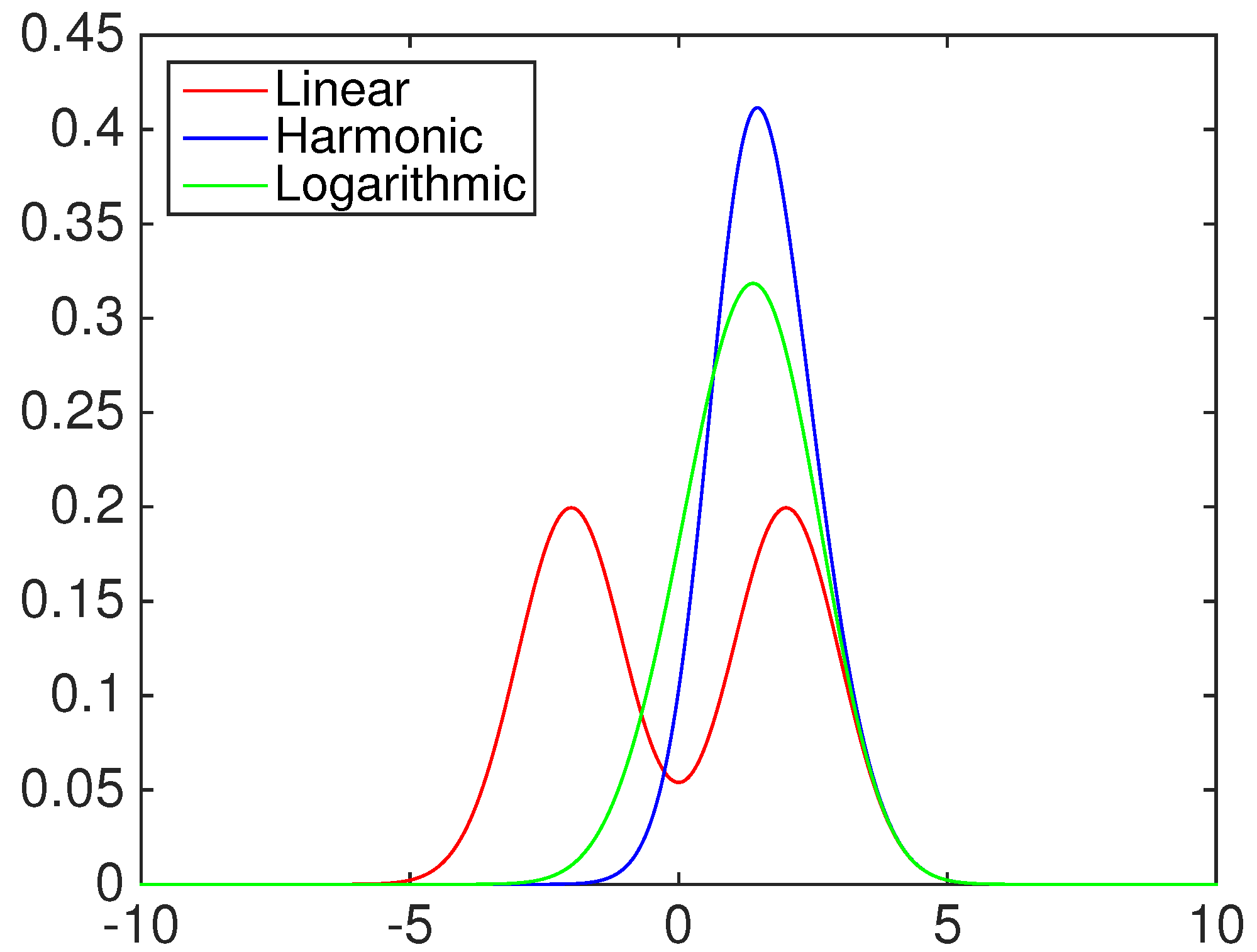
where $\mathbf{p}=(p_1,p_2,p_3)\in {\Delta }_3$. Moreover, we assume that the set of predictive models includes two normal distributions: $\mathcal{N}(-1,1)$ and $\mathcal{N}(0.5,3)$. The distributions of the combination schemes compared in our simulation experiments are:

• the equally-weighted model (EW):

  $$\begin{array}{cc}\hfill H_{1t}(y,\omega )& =\omega F\left(y\right|-1,1)+(1-\omega \left)F\right(y|0.5,3),\hfill \\ \hfill H_{2t}(y,\omega )& =\omega {\left(F\left(y\right|-1,1)\right)}^{-1}+(1-\omega ){\left(F\left(y\right|0.5,3)\right)}^{-1},\hfill \\ \hfill H_{3t}(y,\omega )& =exp\left(\omega log\left(F\right(y|-1,1))+(1-\omega )log(F\left(y\right|0.5,3\left)\right)\right),\hfill \end{array}$$

  where ω is the combination weight equal to $1/2$. $H_{1t},H_{2t},H_{3t}$ correspond to Equations (3)–(5), for linear, harmonic and logarithmic pool, respectively, when $K=2$;
• the beta calibration model (BC1):

  $$\begin{array}{c}\hfill G_{mt}\left(y\right|\theta )=B_{{\alpha }_1,{\beta }_1}\left(H_{mt}\left(y\right|{\omega }_1)\right)\end{array}$$

  where $\theta =({\alpha }_1,{\beta }_1,{\omega }_1)$, and $H_{mt}\left(y\right|\omega )$, with $\omega ={\omega }_1$, is defined by Equations (3)–(5);
• the two-component beta mixture calibration model (BC2):

  $$\begin{array}{c}\hfill G_{mt}\left(y\right|\theta )=\rho B_{{\alpha }_1,{\beta }_1}\left(H_{mt}\left(y\right|{\omega }_1)\right)+(1-\rho )B_{{\alpha }_2,{\beta }_2}\left(H_{mt}\left(y\right|{\omega }_2)\right),\end{array}$$

  where $\theta =(\rho ,{\alpha }_1,{\alpha }_2,{\beta }_1,{\beta }_2,{\omega }_1^{{}^{\prime }},{\omega }_2^{{}^{\prime }})$ and $H_{mt}\left(y\right|\omega )$ is the same as in the BC1 model.

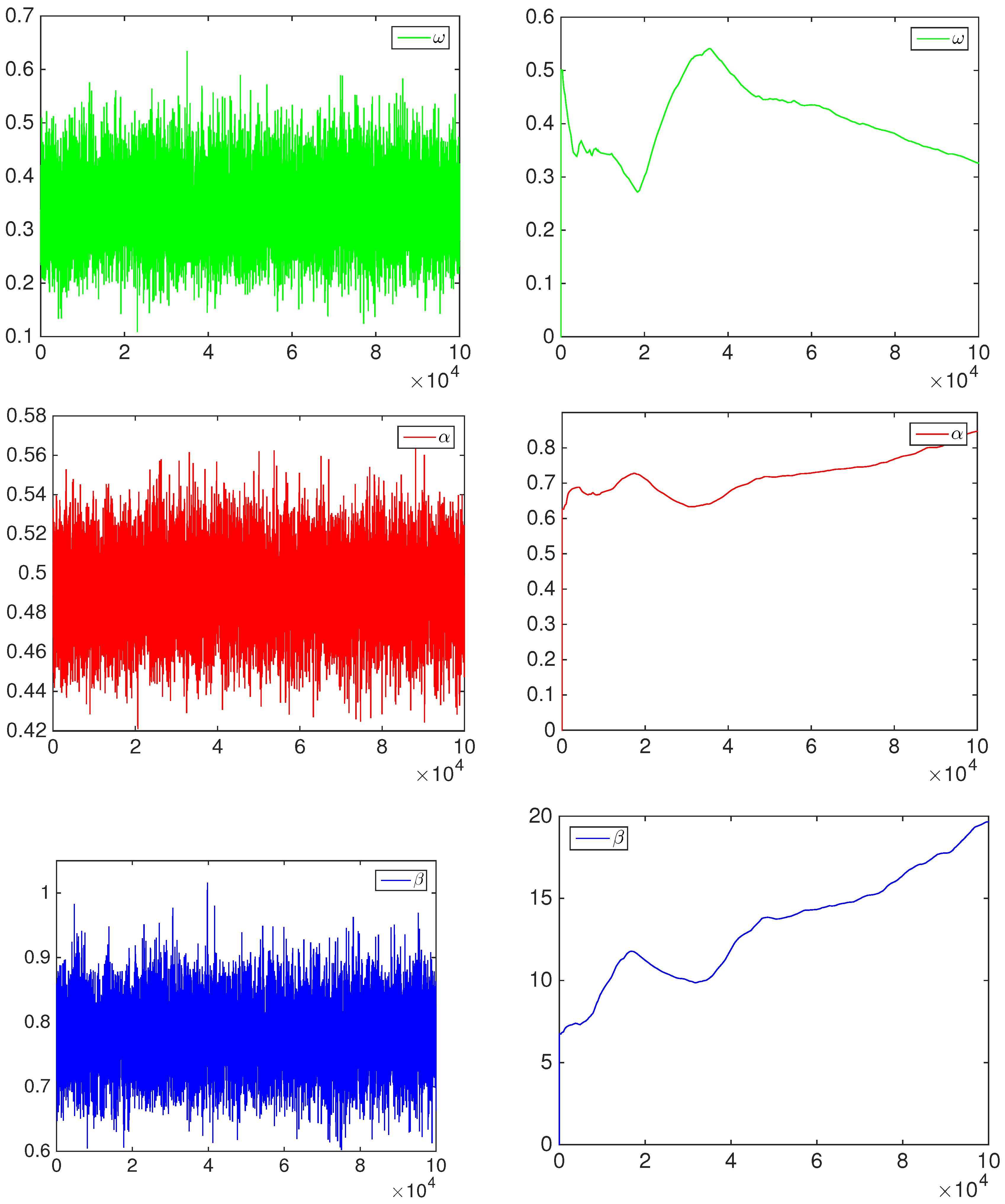
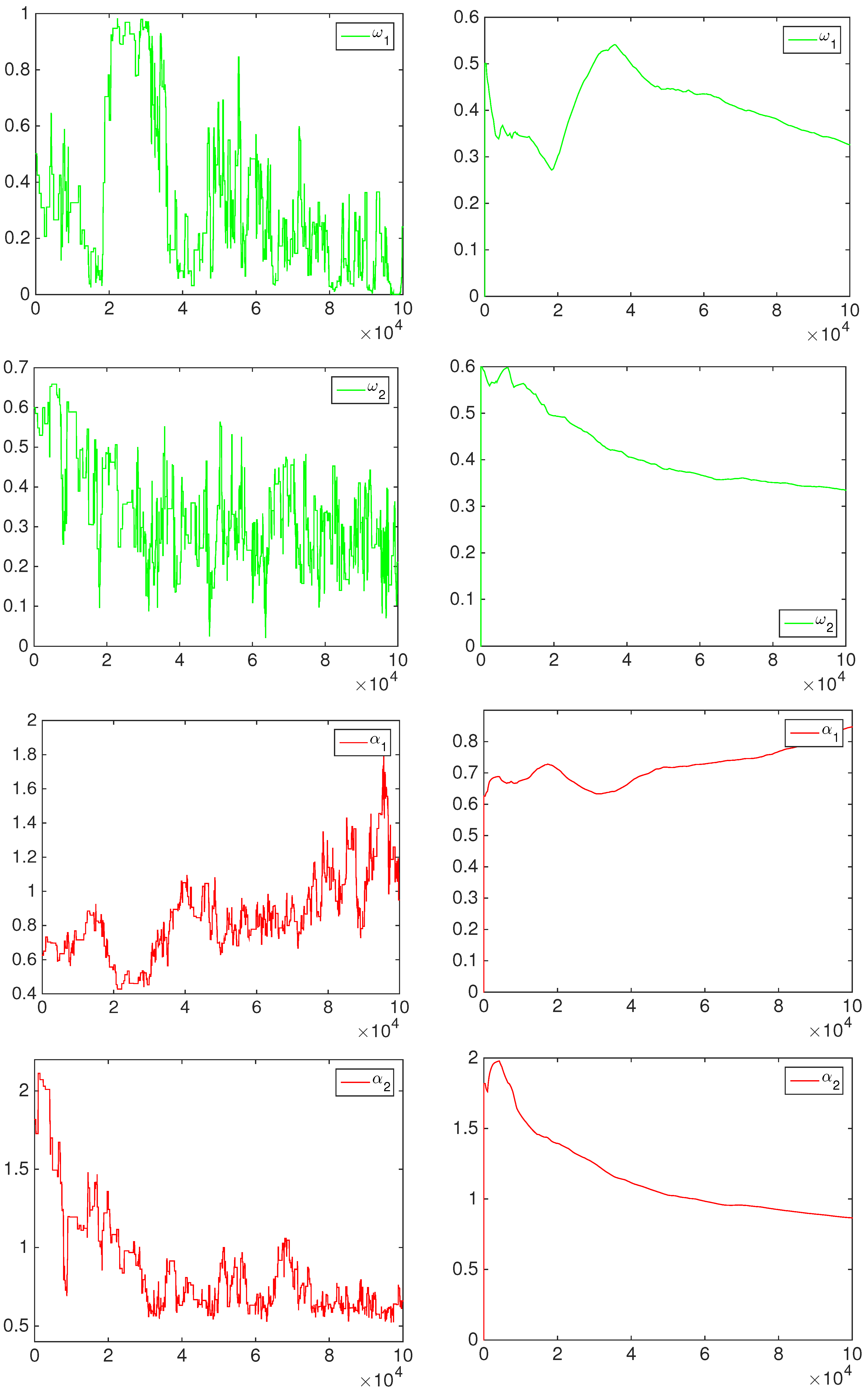
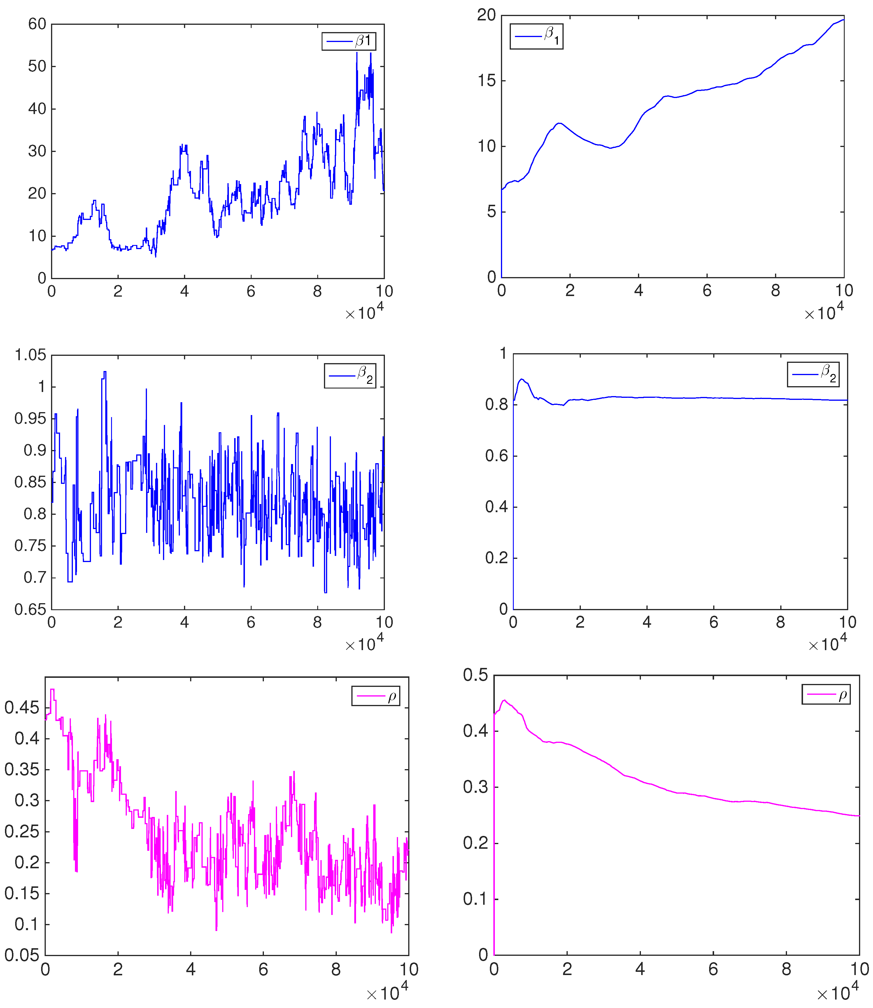
The posterior approximation is based on a set of 50,000 MCMC iterations after a burn-in period of 50,000 iterations. An example of MCMC output is given in the Appendix. In order to reduce the dependence in the samples, we thin out every 50th draw after the burn-in period. Therefore, we obtain 1000 samples, which are used to approximate all of the posterior quantities of interest.

The posterior means of the BC1 and BC2 parameters (represented by the vector θ) are reported in

Table 1. Parameter estimates in the linear combination model for different choices of the mixture probabilities $\mathbf{p}$ of the data-generating process.

p	(1/5, 1/5, 3/5)		(1/7, 1/7, 5/7)		(3/5, 1/5, 1/5)		(5/7, 1/7, 1/7)
$\mathit{\theta }$	BC1	BC2	BC1	BC2	BC1	BC2	BC1	BC2
${\alpha }_1$	0.755	3.293	0.921	6.970	0.461	0.452	0.496	0.650
${\beta }_1$	0.642	0.953	0.639	0.937	0.816	3.744	0.812	0.876
${\omega }_1$	0.015	0.191	0.000	0.500	0.256	0.925	0.342	0.230
${\alpha }_2$		0.692		0.665		0.550		0.707
${\beta }_2$		3.093		0.713		0.827		13.033
${\omega }_2$		0.150		0.233		0.063		0.315
ρ		0.697		0.512		0.215		0.806

for the linear combination models, in

Table 2. Parameter estimates in the harmonic combination model for different choices of the mixture probabilities $\mathbf{p}$ of the data-generating process.

p	(1/5, 1/5, 3/5)		(1/7, 1/7, 5/7)		(3/5, 1/5, 1/5)		(5/7, 1/7, 1/7)
$\mathit{\theta }$	BC1	BC2	BC1	BC2	BC1	BC2	BC1	BC2
${\alpha }_1$	0.744	7.026	0.906	7.775	0.416	0.383	0.457	0.457
${\beta }_1$	0.634	0.878	0.632	1.013	0.755	0.827	0.747	0.778
${\omega }_1$	0.042	0.529	0.024	0.456	0.363	0.734	0.507	0.511
${\alpha }_2$		0.615		0.665		3.720		0.462
${\beta }_2$		0.929		0.651		1.133		0.734
${\omega }_2$		0.380		0.302		0.093		0.474
ρ		0.453		0.415		0.824		0.456

for the harmonic combination models and in

Table 3. Parameter estimates in the logarithmic combination model for different choices of the mixture probabilities $\mathbf{p}$ of the data-generating process.

p	(1/5, 1/5, 3/5)		(1/7, 1/7, 5/7)		(3/5, 1/5, 1/5)		(5/7, 1/7, 1/7)
$\mathit{\theta }$	BC1	BC2	BC1	BC2	BC1	BC2	BC1	BC2
${\alpha }_1$	0.751	7.062	0.917	6.514	0.441	2.587	0.469	2.180
${\beta }_1$	0.639	0.950	0.640	0.966	0.764	1.109	0.753	0.869
${\omega }_1$	0.018	0.517	0.000	0.431	0.370	0.031	0.465	0.411
${\alpha }_2$		0.578		0.645		0.367		0.515
${\beta }_2$		0.823		0.680		0.875		2.770
${\omega }_2$		0.426		0.379		0.843		0.423
ρ		0.484		0.510		0.274		0.389

for the logarithmic combination models, according to $p_i$. In the tables, ${\alpha }_1$ and ${\beta }_1$ stand for the parameters of the beta distribution and ${\omega }_1$ for the combination weight in the BC1 model and in the first component of the BC2 model, while the parameters of the second component of BC2 are referred to as ${\alpha }_2$, ${\beta }_2$ and ${\omega }_2$.

Generally, BC2 models build more flexible predictive cdf: in most of the cases presented, the BC1 models do not take into account the first predictive distribution function ($F_1$), while BC2 weights more the first one than the second predictive cdf, with few exceptions. Comparing pooling schemes, no clear tendency appears from the tables.

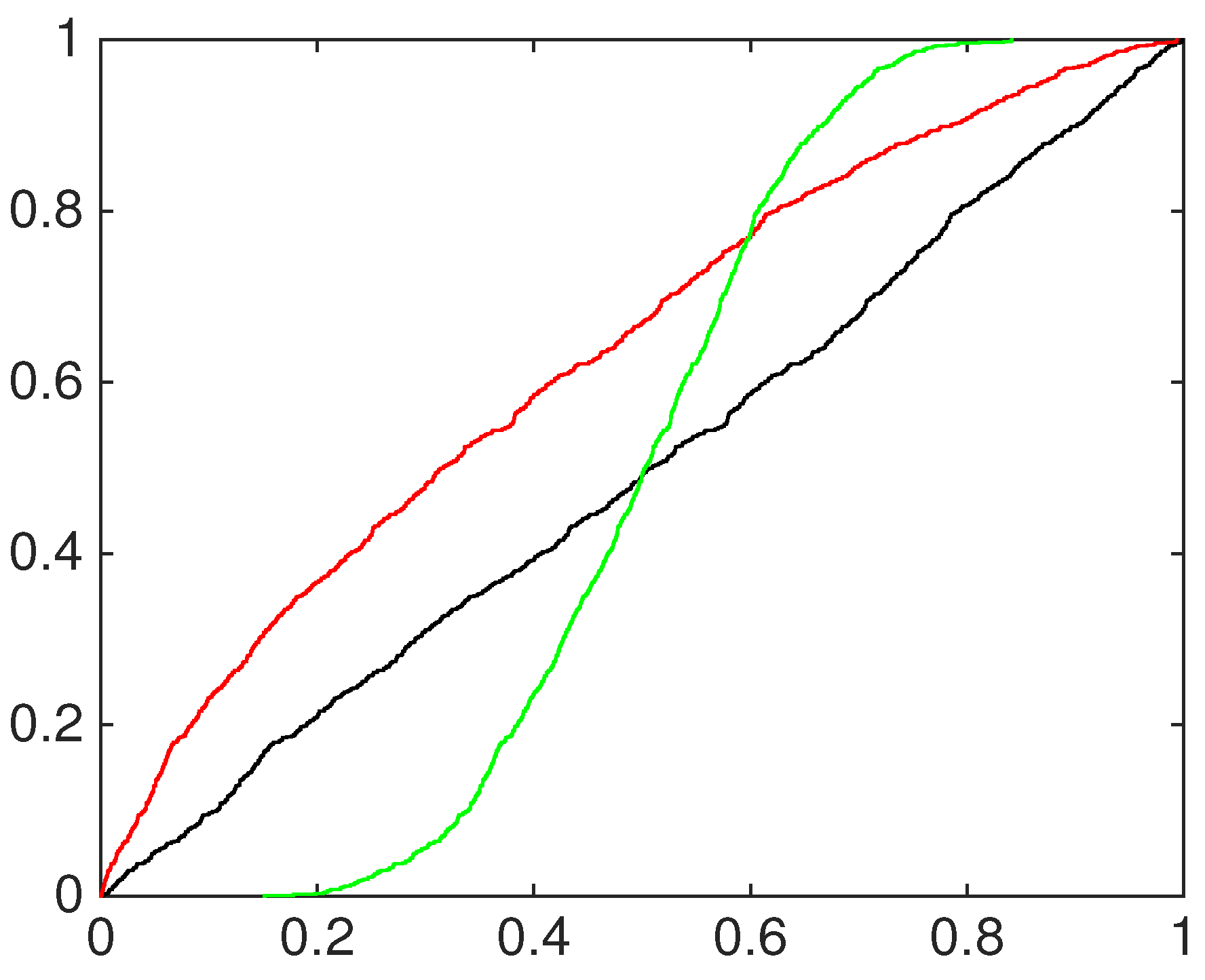
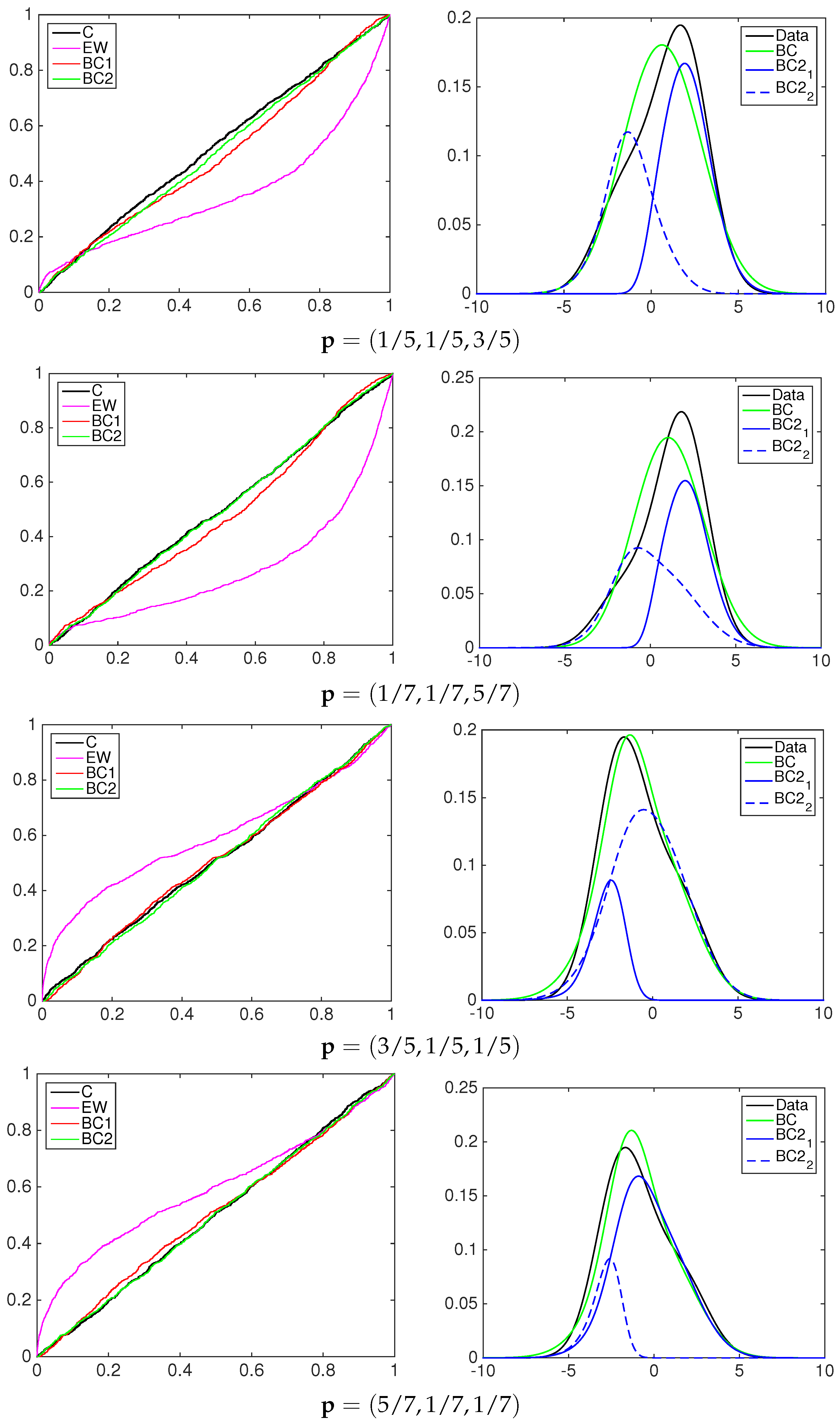
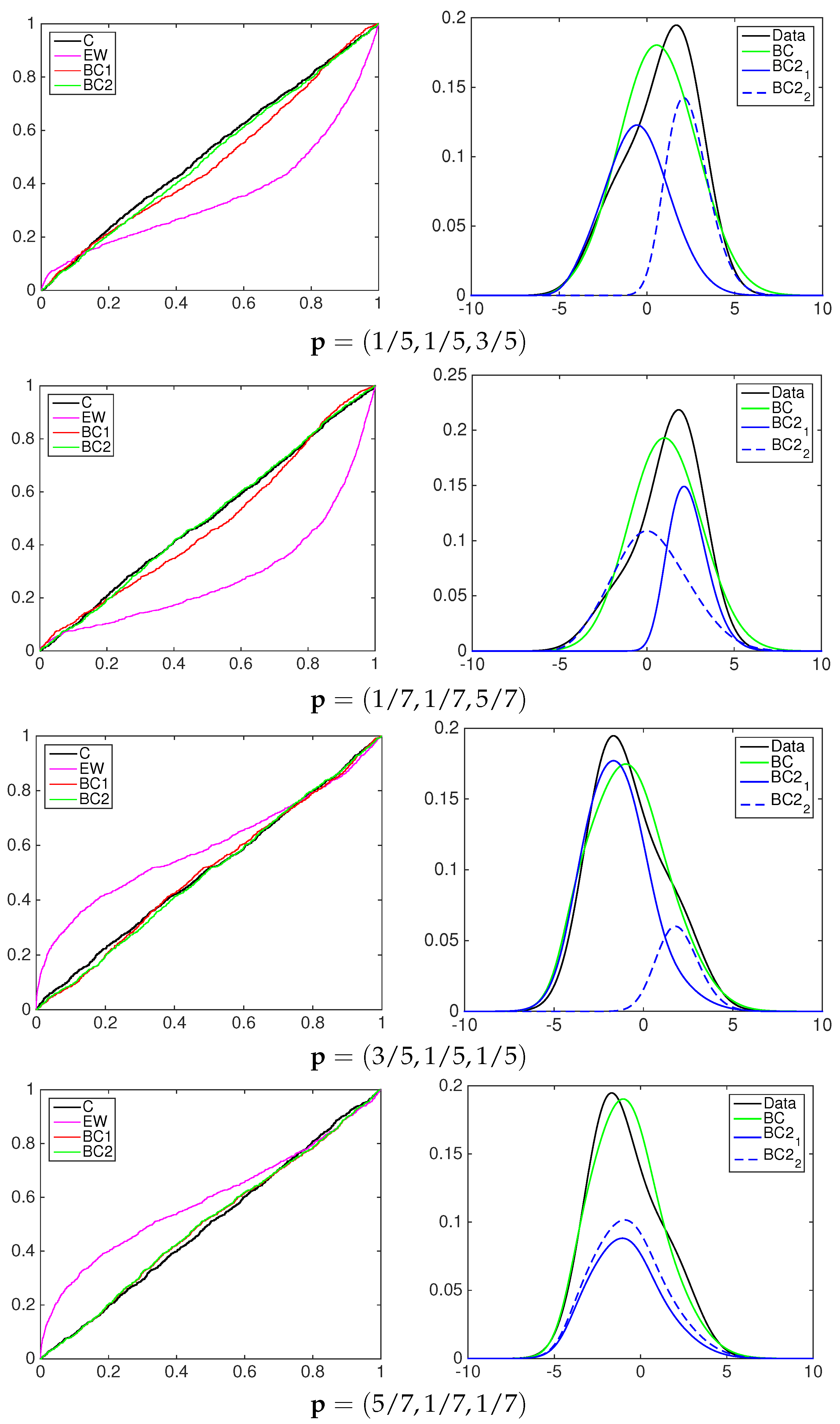
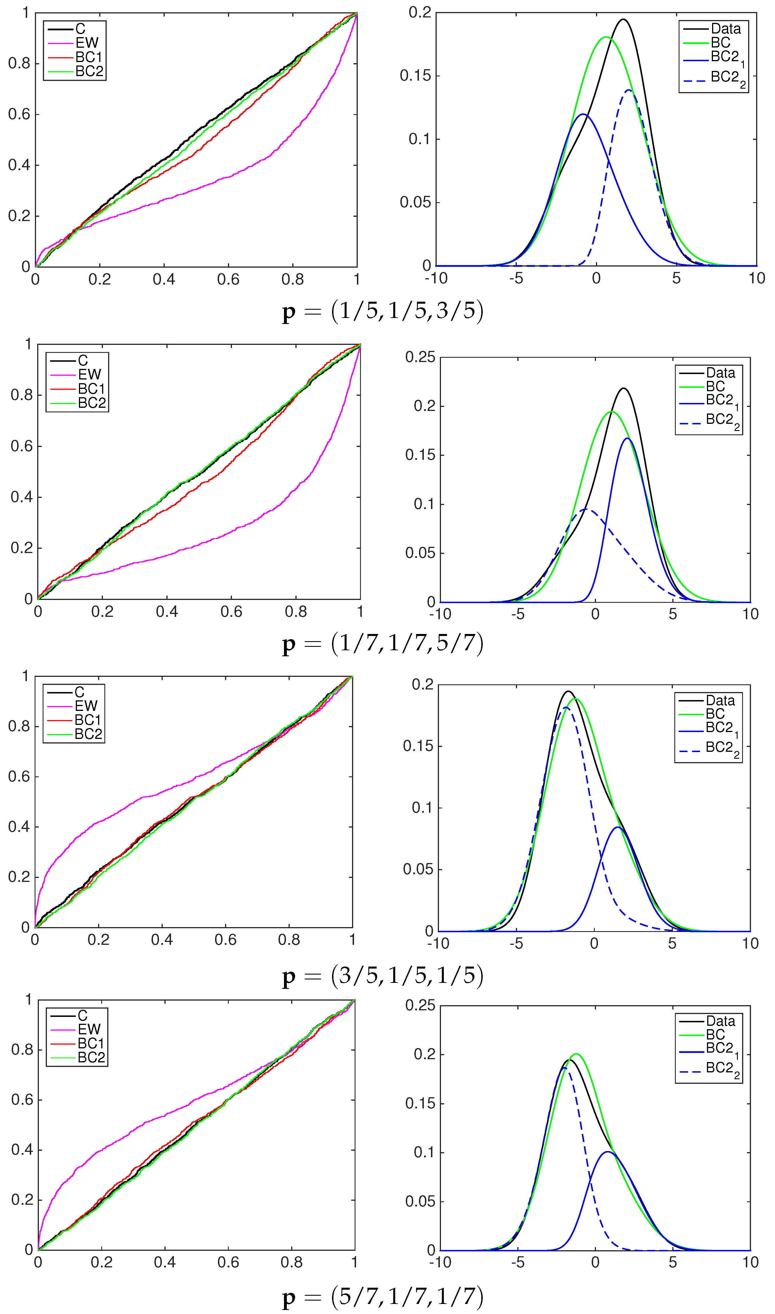
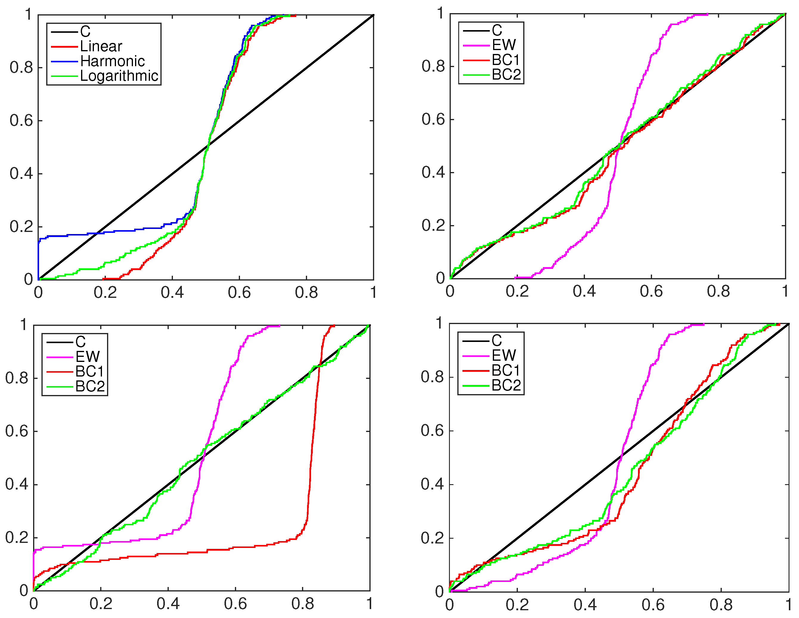
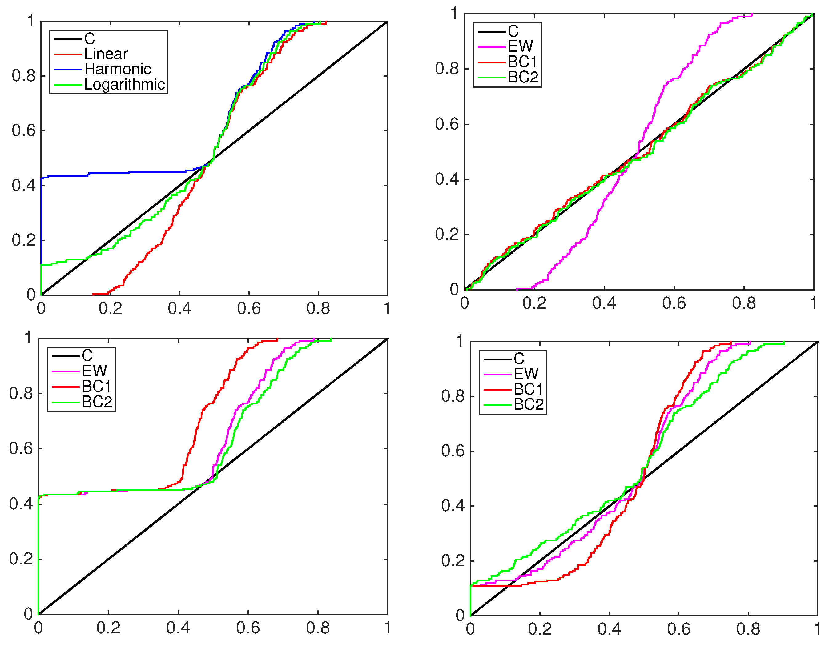
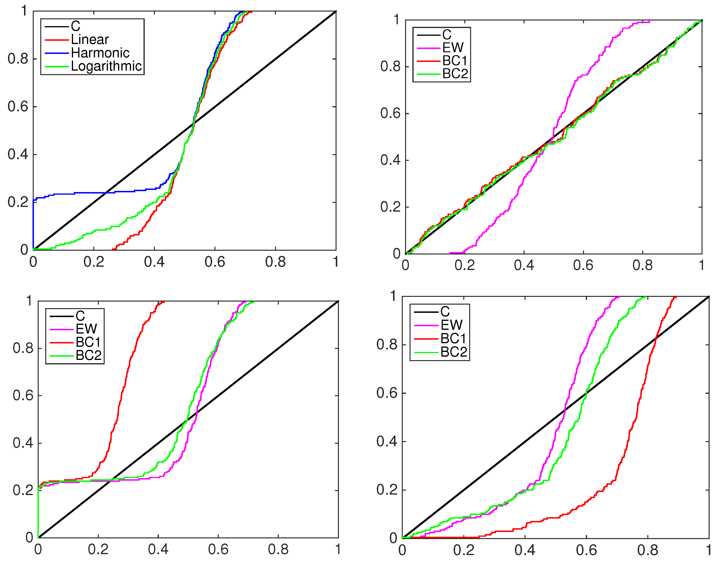
A graphical inspection of PIT cumulative density functions of the three models is proposed to compare them to the simulated data to be predicted; see the left column in Figure 5, Figure 6 and Figure 7. In all of the experiments the PITs of the equally-weighted model (magenta line) lack the ability to predict acceptably the standard uniform cdf of the data simulated by a mixture of normal distributions.

The beta-transformed models (red line) predict the uniformity better than the EQ models, but they overestimate or underestimate the black line mainly in the central part of the support. In all of the pooling schemes used, the beta mixture models provide the closest calibrated cdfs to the uniform one, being able to achieve better flexibility among the others.

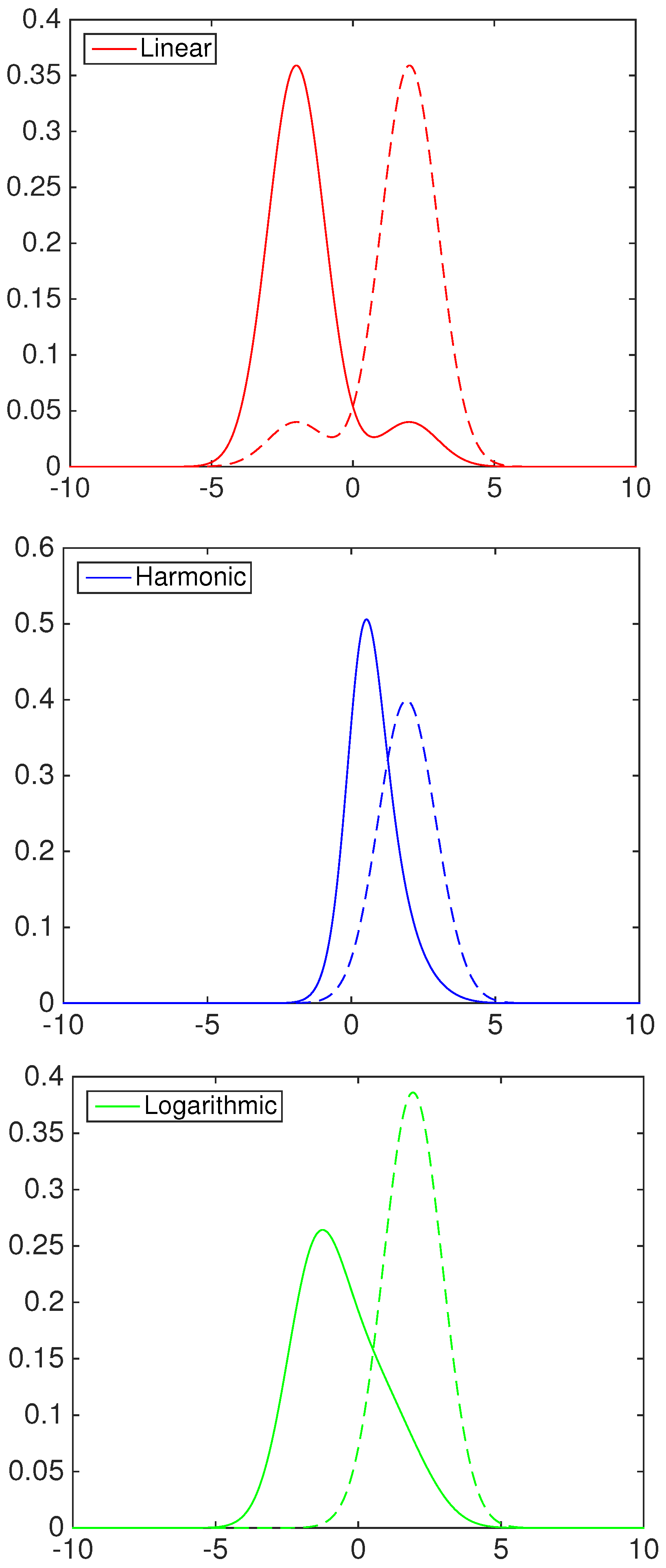
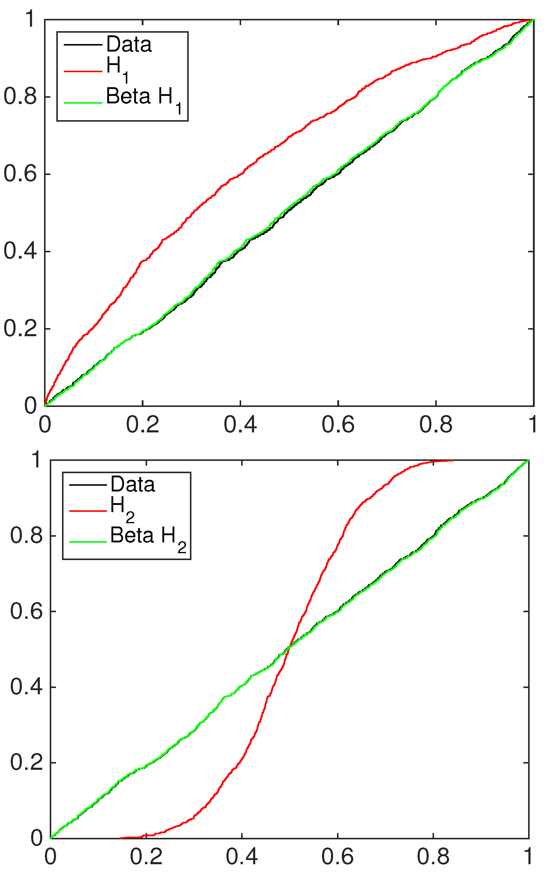
To highlight the behavior of the two-component beta mixture, the right column of Figure 5, Figure 6 and Figure 7 shows the contribution in the calibration process of each element. As an example, consider the first panel in Figure 5, the BC1 and BC2 models with linear pooling. The solid blue line represents the pdf of the first component of the mixture, the dashed blue line the second component. The multimodality of the data is explained by two predictive functions: the first mixture component, denoted by BC2${}_1$, calibrates mainly the predictive density over the positive part of the support; the second mixture component, denoted by BC2${}_2$, calibrates the density over the negative part. Table 1 reports the following values for the weight ω: ${\omega }_1=0.5390$ and ${\omega }_2=0.8700$. This means that both components weight the first model in the pool more, i.e., $\mathcal{N}(0.5,3)$.

In conclusion, our simulation exercises find that the result presented in [19] for the calibration and linear pooling combination of predictive densities is valid for and can be extended to other pooling schemes, including the logarithmic pooling and the harmonic pooling. Moreover, no clear preference for one combination scheme appears from our examples.

4.2. Financial Application: Standard&Poors500 Index

We consider S&P500 daily percent log returns from 1 January 2007–31 December 2009; an updated version of the database used in [14,18,35]. The price series $\left\{y_t\right\}$ were constructed assembling data from different sources: the WRDS database; Thompson/Data Stream; the total number of returns in the sample is $t=784$. Many investors try to replicate the performance of the S&P500 Index with a set of stocks, not necessarily identical to those included in the index. Casarin et al. [21] individuates 3712 stocks quoted in the NYSE and NASDAQ eligible for this purpose, whose 1883 satisfy the control for liquidity (i.e., each stock has been traded a number of days corresponding to at least 40% of the sample size).

Then, a density forecast for each of the stock prices is produced by the following equations:

$$\begin{array}{}\mathrm{(20)}& \hfill y_{it}& =& c_i+{\kappa }_{it}{\zeta }_{it}\hfill \mathrm{(21)}& \hfill {\kappa }_{it}^2& =& {\theta }_{i0}+{\theta }_{i1}{\zeta }_{i,t-1}^2+{\theta }_{12}{\kappa }_{i,t-1}^2\hfill \end{array}$$

where $y_{it}$ is the log return of stock $i=1,\cdots ,1883$, at day t; ${\zeta }_{i,t-1}\sim \mathcal{N}(0,1)$ and ${\zeta }_{i,t-1}\sim \mathcal{T}\left({\nu }_i\right)$ for the normal and t-Student cases, respectively. Both models produce 784 one day ahead density forecasts from 1 January 2007–31 December 2009 by substituting the maximum likelihood (ML) estimates for the unknown parameters $(c_i,{\theta }_{i0},{\theta }_{i1},{\theta }_{i2},{\nu }_i)$ (for further details, please refer to [21]).

The major contribution of this technique is the construction of a sequential cluster analysis for our forecasts. The work in [21] computes two clusters: one for normal GARCH(1,1) models and another one for t-GARCH(1,1). Then, we obtain a combined forecast of the S&P500 Index combining and calibrating the two classes of predictive distribution functions, i.e., GARCH(1,1) and t-GARCH(1,1), through the equally-weighted, the beta-calibrated and the two-component beta mixture models with linear, harmonic and logarithmic pooling schemes.

The clustered weights are assumed to be one and defined by:

$${\omega }_i=\left\{\begin{array}{cc}\frac{\omega }{3766},\hfill & i\le 1883\hfill \\ \frac{1-\omega }{3766},\hfill & i>1883\hfill \end{array}\right.$$

where 3766 is the total number of predictive distribution functions: 1883 belonging to the class GARCH(1,1) and 1883 to the class t-GARCH(1,1). That is, the combination model gives weight ${\omega }_i/1883$ to the class of GARCH(1,1) (first 1883 models) and $1-{\omega }_i/1883$ to the class of t-GARCH(1,1) (second 1883 models). The stage is open to further extensions, suggesting a less restricting weighting system.

The period taken into account is particularly interesting because it includes the U.S. financial crisis. Our analysis considers three subsamples, of 200 observations each, representing three periods with different features. The time from 1 January 2007–5 October 2007 is defined as a tranquil period, and the predictability of the index could be hypothesized better than the one from 20 June 2008–26 March 2009 during which the financial crisis developed: here, one can expect that the high volatility makes it more difficult to predict the returns. Finally, the third subsample includes data from 27 March 2009–31 December 2009, the post-crisis period. We aim to inquire if some difficulties in the forecastability and forecast calibration are still present in the post-crisis period. The two classes of predictive density functions, GARCH(1,1) and t-GARCH(1,1), are combined and calibrated through the following models: the equally-weighted (EW) model, the beta-calibrated (BC1) model and the two mixture beta-calibrated (BC2) model. For each model, the three combination schemes are considered: linear, harmonic and logarithmic.

The sequential estimation and combination of the models have been conducted on a cluster multiprocessor system, which consists of four nodes; each comprises four Xeon E5-4610 v2 2.3-GHz CPUs, with eight cores, 256 GB ECC PC3-12800R RAM, Ethernet 10 Gbit and 20-TB hard disk system with Linux. The code has been implemented in MATLAB (see [36]), and the parallel computing makes use of the MATLAB parallel computing toolbox. The parallel implementation of the sequential estimation exercise allows us to obtain the results in 36 hours with a computational gain of the parallel over the sequential implementation of 120 hours.

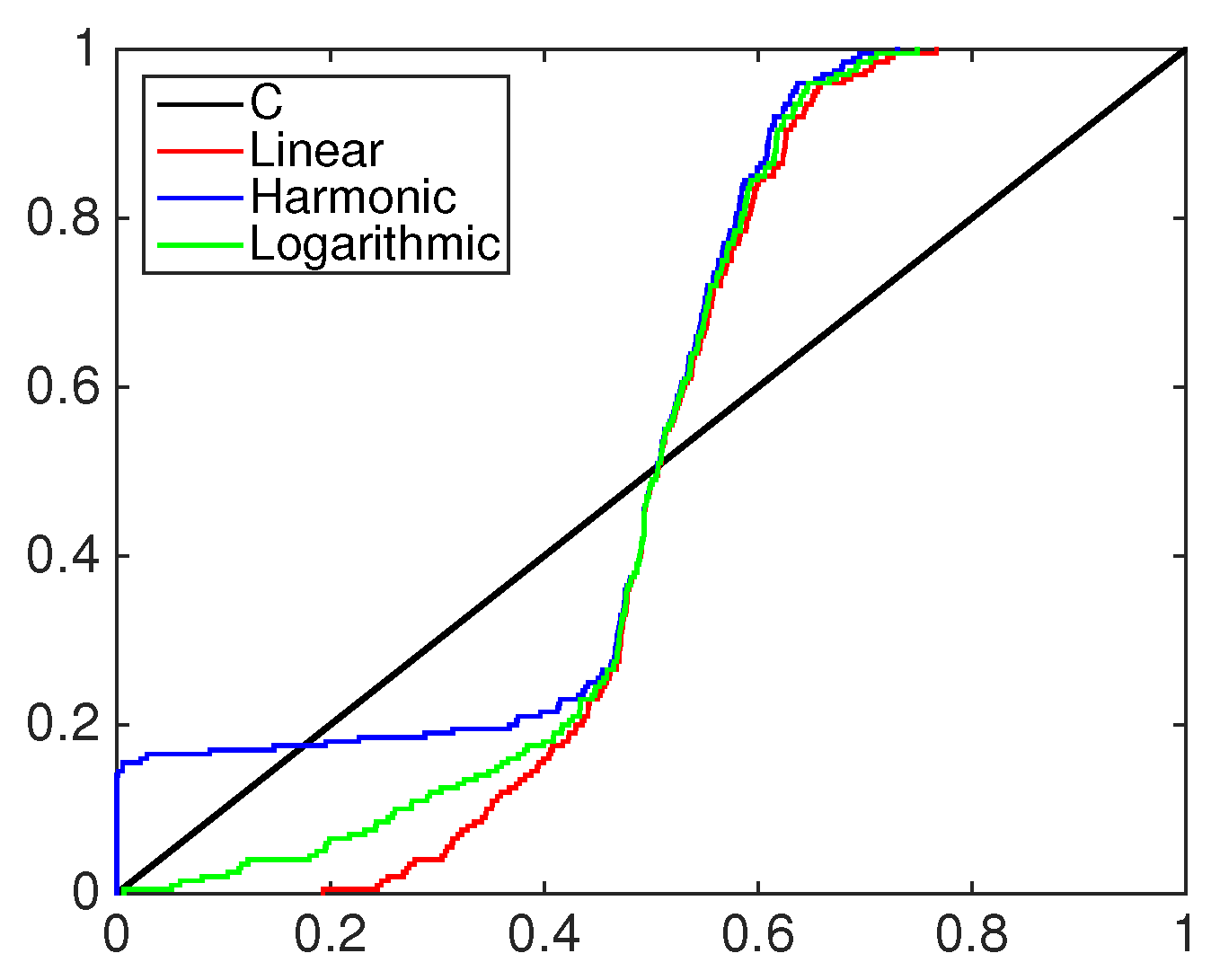
Figure 8 displays a comparison through PITs of linear, harmonic and logarithmic pools when those are combined with the equally-weighted model and the 45 degree line, which represents the PITs for the unknown ideal model. Linear, harmonic and logarithmic pools have the same behavior in the center part of the support; the differences among them are mainly in the tails, in particular in the left one. With respect to the linear and logarithmic scheme, indeed, the harmonic pool (blue line) underestimates more often the frequency of the observations in the tails. The scheme closer to the 45 degree line is the harmonic one, thanks to its better performance in predicting tail events.

For the first 200 days, from 1 January 2007–10 October 2007, where the volatility is roughly the same, the posterior means of the BC1 and BC2 parameters (represented by the vector θ) are reported in

Table 4. Parameter estimates in the different combination models for the pre-crisis data subsample: 1 January 2007–5 October 2007.

P	Linear		Harmonic		Logarithmic
$\mathit{\theta }$	BC1	BC2	BC1	BC2	BC1	BC2
${\alpha }_1$	5.840	0.000	0.084	17.573	2.468	34.692
${\beta }_1$	5.807	0.000	0.371	15.114	2.867	34.462
${\omega }_1$	1.000	0.000	1.000	0.863	1.000	0.706
${\alpha }_2$		5.812		0.020		1.781
${\beta }_2$		5.651		0.466		2.166
${\omega }_2$		1.000		0.199		0.93
ρ		0.000		0.7926		0.269

,

Table 5. Parameter estimates in the different combination models for the in-crisis data subsample: 20 June 2008–26 March 2009.

P	Linear		Harmonic		Logarithmic
$\mathit{\theta }$	BC1	BC2	BC1	BC2	BC1	BC2
${\alpha }_1$	7.025	278.600	0.977	0.944	0.974	1.010
${\beta }_1$	6.646	803.260	0.865	1.014	1.292	1.018
${\omega }_1$	1.000	1.000	0.740	0.263	0.821	0.031
${\alpha }_2$		6.760		0.975		1.131
${\beta }_2$		6.334		1.010		0.972
${\omega }_2$		1.000		0.247		0.298
ρ		0.000		0.000		0.000

and

Table 6. Parameter estimates in the different combination models for the pre-crisis data subsample: 27 March 2009–31 December 2009.

P	Linear		Harmonic		Logarithmic
$\mathit{\theta }$	BC1	BC2	BC1	BC2	BC1	BC2
${\alpha }_1$	6.542	47110.000	1.031	0.972	1.127	1.007
${\beta }_1$	6.071	0.000	0.419	0.942	2.275	1.066
${\omega }_1$	1.000	1.000	0.823	0.967	0.186	0.406
${\alpha }_2$		6.710		1.039		0.891
${\beta }_2$		6.307		0.938		1.015
${\omega }_2$		1.000		0.920		0.921
ρ		0.000		0.000		0.000

. Here, ${\alpha }_1$ and ${\beta }_1$ stand for the parameters of the beta distribution in the estimated BC1 model and in the first component of the BC2 model, while the second component of BC2 is referred to as ${\alpha }_2$ and ${\beta }_2$.

In all of the cases presented, the estimated BC1 models give zero weight to the class of t-GARCH(1,1) models, as well as the fist component of the beta mixture (BC2); while the second component of the BC2 in the harmonic and logarithmic cases weights the class of t-GARCH(1,1) models more than the class of GARCH(1,1) models. To better understand the effect of these parameter estimates, a graphical inspection of PITs is reported in Figure 9, Figure 10 and Figure 11, for the pre-crisis, in-crisis and post-crisis period respectively.

In all examples, the equally-weighted model (magenta line) lacks the ability to predict acceptably the ideal standard uniform cdf; see Figure 9, Figure 10 and Figure 11. Just in one case, the linear one, both BC1 and BC2 perform well, providing the closest calibration to the uniform one, being able to achieve better flexibility for all of the time periods analyzed. In the harmonic and logarithmic cases, the BC1 model lacks the ability to calibrate the class of GARCH(1,1) and the class of t-GARCH(1,1) models, fitting even worsen than the equal weight model. However, a satisfactory calibration is obtained by the BC2 model, even if not as good as that achieved by the linear pool. This is confirmed for all if the periods in our sample, even if the PITs’ calibration gets worse in the crisis and post-crisis phases, highlighting some difficulties in being flexible. However, the linear pooling achieves good calibrated forecasts in both beta combination models; if the pool employed is chosen among the harmonic and the logarithmic schemes, satisfactory results are provided by the two-component beta mixture model.

In conclusion, we prove that the result in [19] for the beta mixture calibration and linear combination of predictive densities is still valid when harmonic and logarithmic combination schemes are applied.

5. Conclusions

This paper applies a Bayesian beta mixture model to derive a combined and calibrated density function using random calibration functionals and random combination weights. It compares linear, harmonic and logarithmic pooling in the combination approach in simulation examples with multimodal densities and an application with a large set of stock market data.

The results show that the three combination pools allow for achieving well-calibrated forecasts, and no clear preference for one of them appears. However, in the application to the daily log returns of the S&P500 Index, the linear pooling together with beta mixture calibration achieves the best results in terms of calibrated forecast.

References

1. G.A. Barnard. “New methods of quality control.” J. R. Stat. Soc. Ser. A 126 (1963): 255–259. [Google Scholar] [CrossRef]
2. H.V. Roberts. “Probabilistic prediction.” J. Am. Stat. Assoc. 60 (1965): 50–62. [Google Scholar] [CrossRef]
3. J.A. Hoeting, D. Madigan, A.E. Raftery, and C.T. Volinsky. “Bayesian model averaging: A tutorial.” Stat. Sci. 14 (1999): 382–417. [Google Scholar]
4. J.M. Bates, and C.W.J. Granger. “Combination of forecasts.” Oper. Res. Q. 20 (1969): 451–468. [Google Scholar] [CrossRef]
5. A. Timmermann. “Forecast combinations.” In Handbook of Economic Forecasting. Edited by G. Elliot, C. Granger and A. Timmermann. North-Holland, The Netherlands: Elsevier, 2006, Chapter 4; Volume 1, pp. 135–196. [Google Scholar]
6. V. Corradi, and N.R. Swanson. “Predictive density and conditional confidence interval accuracy tests.” J. Econom. 135 (2006): 187–228. [Google Scholar] [CrossRef]
7. S.G. Hall, and J. Mitchell. “Combining density forecasts.” Int. J. Forecast. 23 (2007): 1–13. [Google Scholar] [CrossRef]
8. J. Mitchell, and S.G. Hall. “Evaluating, comparing and combining density forecasts using the KLIC with an application to the Bank of England and NIESER “fan” charts of inflation.” Oxf. Bull. Econ. Stat. 67 (2005): 995–1033. [Google Scholar] [CrossRef]
9. K.F. Wallis. “Combining density and interval forecasts: A modest proposal.” Oxf. Bull. Econ. Stat. 67 (2005): 983–994. [Google Scholar] [CrossRef]
10. C. Genest, and J. Zidek. “Combining probability distributions: A critique and an annotated bibliography.” Stat. Sci. 1 (1986): 114–148. [Google Scholar] [CrossRef]
11. M. Stone. “The opinion pool.” Ann. Math. Stat. 32 (1961): 1339–1342. [Google Scholar] [CrossRef]
12. M.H. DeGroot, A.P. Dawid, and J. Mortera. “Coherent combination of experts’ opinions.” Test 4 (1995): 263–313. [Google Scholar]
13. M.H. DeGroot, and J. Mortera. “Optimal linear opinion pools.” Manag. Sci. 37 (1991): 546–558. [Google Scholar] [CrossRef]
14. J. Geweke, and G. Amisano. “Optimal prediction pools.” J. Econom. 164 (2011): 130–141. [Google Scholar] [CrossRef]
15. R. Ranjan, and T. Gneiting. “Combining probability forecasts.” J. R. Stat. Soc. Ser. B 72 (2010): 71–91. [Google Scholar] [CrossRef]
16. M. Billio, R. Casarin, F. Ravazzolo, and H. van Dijk. “Time-varying combinations of predictive densities using nonlinear filtering.” J. Econom. 177 (2013): 213–232. [Google Scholar] [CrossRef] [Green Version]
17. R. Casarin, S. Grassi, F. Ravazzolo, and H. van Dijk. “Parallel sequential Monte Carlo for efficient density combination: The DeCo MATLAB toolbox.” J. Stat. Softw. 68 (2015): 1–30. [Google Scholar] [CrossRef]
18. N. Fawcett, G. Kapetanios, J. Mitchell, and S. Price. “Generalised density forecast combinations.” J. Econom. 188 (2015): 150–165. [Google Scholar] [CrossRef]
19. F. Bassetti, R. Casarin, and F. Ravazzolo. Bayesian Nonparametric Calibration and Combination of Predictive Distributions. Paper Series No. 04/WP/2015; Venice, Italy: University Ca’ Foscari of Venice, Department of Economics, 2015. [Google Scholar]
20. T. Gneiting, and R. Ranjan. “Combining predictive distributions.” Electron. J. Stat. 7 (2013): 1747–1782. [Google Scholar] [CrossRef]
21. R. Casarin, S. Grassi, F. Ravazzolo, and H.K. van Dijk. Dynamic Predictive Density Combinations for Large Datasets. Tinbergen Institute Discussion Paper 15-084/III; Amsterdam, The Netherlands: Tinbergen Institute, 2015. [Google Scholar]
22. K.J. McConway. “Marginalization and linear opinion pools.” J. Am. Stat. Assoc. 76 (1981): 410–415. [Google Scholar] [CrossRef]
23. M. Bacharach. “Group decisions in the face of differences of opinion.” Manag. Sci. 22 (1975): 182–191. [Google Scholar] [CrossRef]
24. R. Laddaga. “Lehrer and the consensus proposal.” Synthese 36 (1977): 473–477. [Google Scholar] [CrossRef]
25. S.C. Hora. “An analytic method for evaluating the performance of aggregation rules for probability densities.” Oper. Res. 58 (2010): 1440–1449. [Google Scholar] [CrossRef]
26. A.P. Dawid. “Intersubjective statistical models.” In Exchangeability in Probability and Statistics. Edited by G. Koch and F. Spizichino. North Holland, Amsterdam, The Netherlands, 1982, pp. 217–232. [Google Scholar]
27. M. Rosenblatt. “Remarks on multivariate transformation.” Ann. Math. Stat. 23 (1952): 1052–1057. [Google Scholar] [CrossRef]
28. A.P. Dawid. “Statistical theory: The prequential approach.” J. R. Stat. Soc. Ser. A 147 (1984): 278–290. [Google Scholar] [CrossRef]
29. T. Gneiting, and R. Ranjan. “Comparing density forecasts using threshold and quantile weighted proper scoring rules.” J. Bus. Econ. Stat. 29 (2011): 411–422. [Google Scholar] [CrossRef]
30. R. Casarin, F. Leisen, G. Molina, and E. Ter-Horst. “Beta markov random field calibration of the term structure of implied risk neutral densities.” Bayesian Anal. 10 (2015): 791–819. [Google Scholar] [CrossRef]
31. C.P. Robert, and J. Rousseau. A Mixture Approach to Bayesian Goodness of Fit. Technical Report 02009; Paris, France: CEREMADE, Université Paris-Dauphine, 2002. [Google Scholar]
32. M. Billio, and R. Casarin. “Beta autoregressive transition Markov-switching models for business cycle analysis.” Stud. Nonlinear Dyn. Econom. 15 (2011): 1–32. [Google Scholar] [CrossRef]
33. N. Bouguila, D. Ziou, and E. Monga. “Practical Bayesian estimation of a finite beta mixture through Gibbs sampling and its applications.” Stat. Comput. 16 (2006): 215–225. [Google Scholar] [CrossRef]
34. R. Casarin, L. Dalla Valle, and F. Leisen. “Bayesian model selection for beta autoregressive processes.” Bayesian Anal. 7 (2012): 1–26. [Google Scholar] [CrossRef]
35. J. Geweke, and G. Amisano. “Comparing and evaluating Bayesian predictive distributions of asset returns.” Int. J. Forecast. 26 (2010): 216–230. [Google Scholar] [CrossRef]
36. The MathWorks, Inc. MATLAB—The Language of Technical Computing. version R2011b; Natick, MA, USA: The MathWorks, Inc., 2011. [Google Scholar]
Figure 1. Density function for linear (red line), harmonic (blue line) and logarithmic (green line) combination models. The combination weight is ω 1 = 0.5 .
Econometrics 04 00017 g001
Figure 2. Combination densities for the three schemes (different rows) for ω 1 = 0.9 (solid lines) and ω 1 = 0.1 (dashed lines).
Econometrics 04 00017 g002
Figure 3. Empirical cdfs of the probability integral transforms (PITs) generated by F 1 (red line), F 2 (green line) and the true model (black line), for the simulated realizations of the variable of interest Y.
Econometrics 04 00017 g003
Figure 4. Beta calibration of F 1 (first row) and F 2 (second row) by using a beta calibration function (i.e., J = 1 ) and the Bayesian estimates of the calibration parameters, that is α 1 = 0.773 and β 1 = 1.352 for F 1 and α 1 = 7.485 and β 1 = 7.477 for F 2 .
Econometrics 04 00017 g004
Figure 5. (Left column): PITs’ cdf for the linear pool at different values of p ; (Right column): contribution of calibration components for BC1 (green) and BC2 (blue), where BC2 1 (solid) is the fist component of the beta mixture in BC2 and BC2 2 (dashed) the second component.
Econometrics 04 00017 g005
Figure 6. (Left column): PITs’ cdf for the harmonic pool at different values of p ; (Right column): contribution of calibration components for BC1 (green) and BC2 (blue), where BC2 1 (solid) is the fist component of the beta mixture in BC2 and BC2 2 (dashed) the second component.
Econometrics 04 00017 g006
Figure 7. (Left column): PITs cdf for the harmonic pool at different values of p ; (Right column): contribution of calibration components for BC1 (green) and BC2 (blue), where BC2 1 (solid) is the fist component of the beta mixture in BC2 and BC2 2 (dashed) the second component.
Econometrics 04 00017 g007
Figure 8. Different behavior of the equally-weighted (EW) model for the three pool schemes applied to the S&P500 daily percent log return.
Econometrics 04 00017 g008
Figure 9. PITs’ cdf of the ideal model C (black line), EW (magenta), BC1 (red) and BC2 (green) for linear (top right), harmonic (bottom left) and logarithmic (bottom right) pools, and the PITs of the EW models (top left) for linear (red), harmonic (blue) and logarithmic (green), in the first data subsample: pre-crisis period.
Econometrics 04 00017 g009
Figure 10. PITs cdf of the ideal model C (black line), EW (magenta), BC1 (red) and BC2 (green) for linear (top right), harmonic (bottom left) and logarithmic (bottom right) pools, and the PITs of the EW models (top left) for linear (red), harmonic (blue) and logarithmic (green), in the second data subsample: in-crisis period.
Econometrics 04 00017 g010
Figure 11. PITs cdf of the ideal model C (black line), EW (magenta), BC1 (red) and BC2 (green) for linear (top right), harmonic (bottom left) and logarithmic (bottom right) pools, and the PITs of the EW models (top left) for linear (red), harmonic (blue) and logarithmic (green), in the third data subsample: post-crisis period.
Econometrics 04 00017 g011
Figure A1. BC1 model ( J = 1 ): 100,000 MCMC samples (left column) and MCMC progressive averages (right column) for the parameters ω 1 , α 1 and β 1 (different rows).
Econometrics 04 00017 g012
Figure A2. BC2 model ( J = 2 ): 100,000 MCMC samples (left column) and MCMC progressive averages (right column) for the parameters ω 1 , ω 2 , α 1 and α 2 (different rows).
Econometrics 04 00017 g013
Figure A3. BC2 model ( J = 2 ): 100,000 MCMC samples (left column) and MCMC progressive averages (right column) for the parameters β 1 , β 2 and ρ (different rows).
Econometrics 04 00017 g014