
Comparative Analysis between Dynamic and Quasi-Steady-State Methods at an Urban Scale on a Social-Housing District in Venice

 ,
,
Abstract
:1. Introduction
2. Materials and Methods
2.1. Dynamic State Simulation by City Energy Analyst Simulation Tool
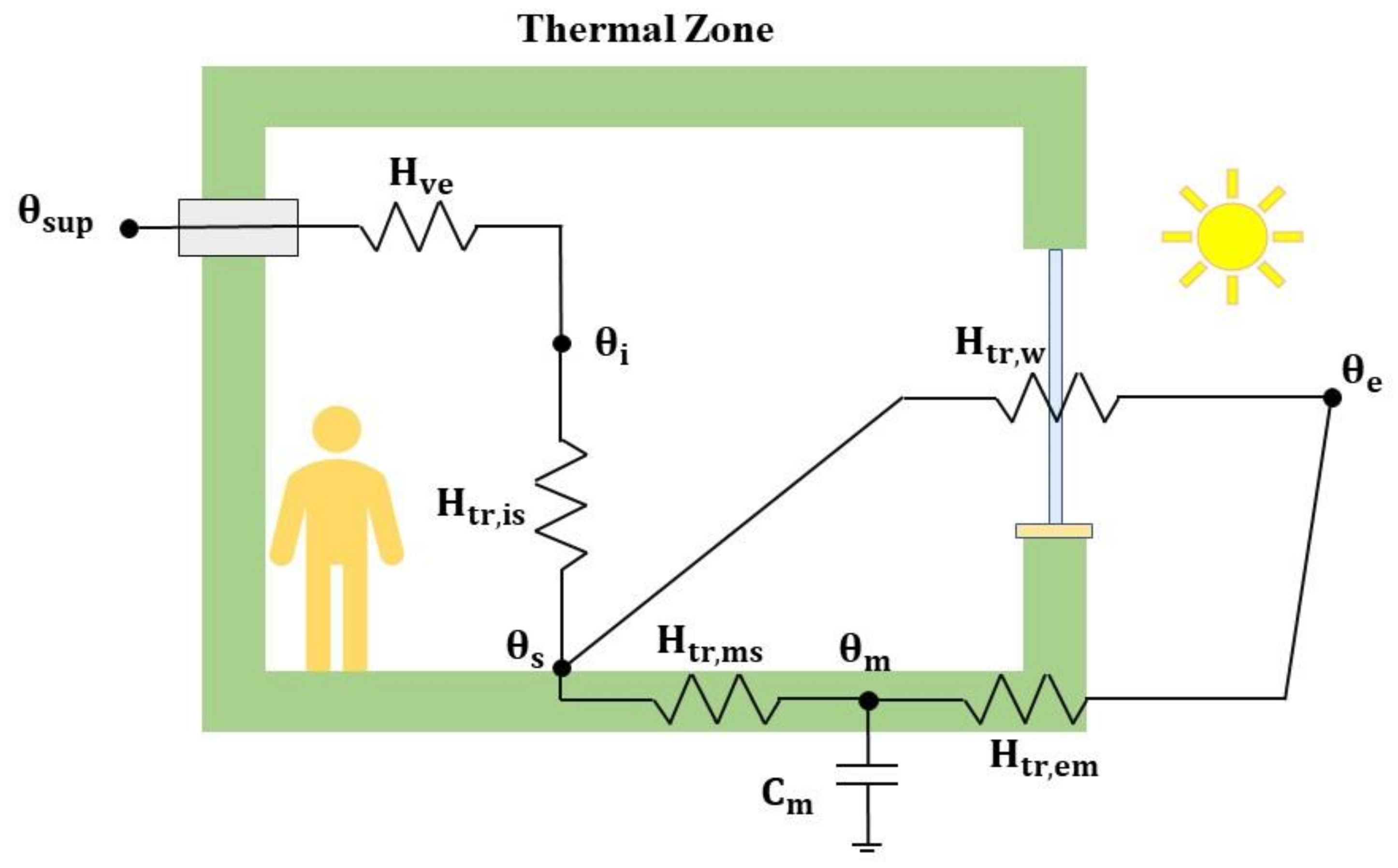
2.2. Dynamic State Simulation by EUReCA
2.3. Quasi-Steady-State Simulation by Spreadsheet Tool
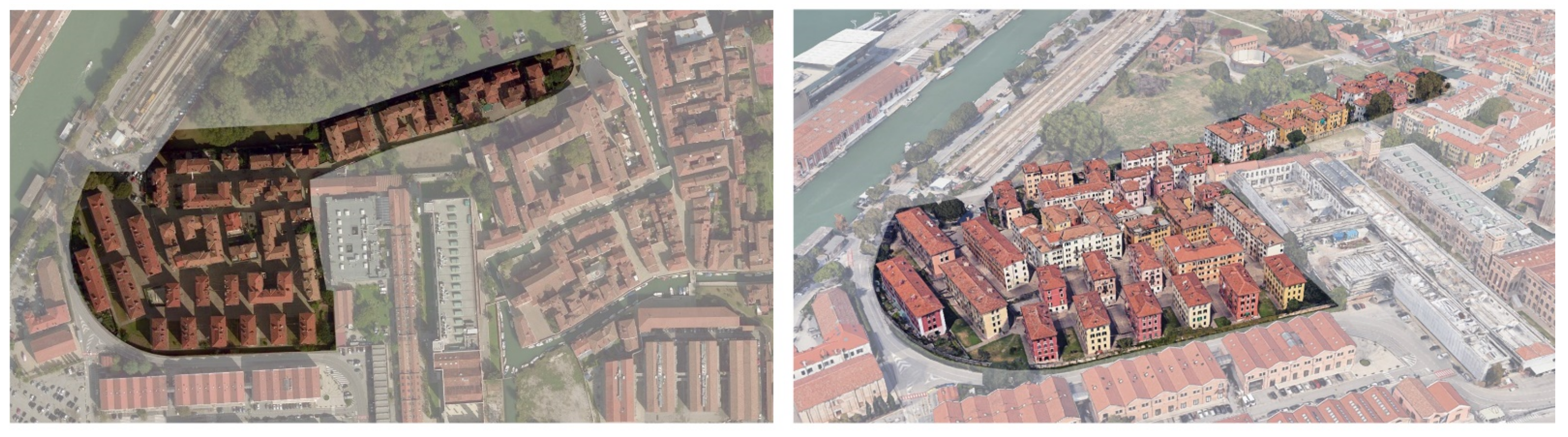
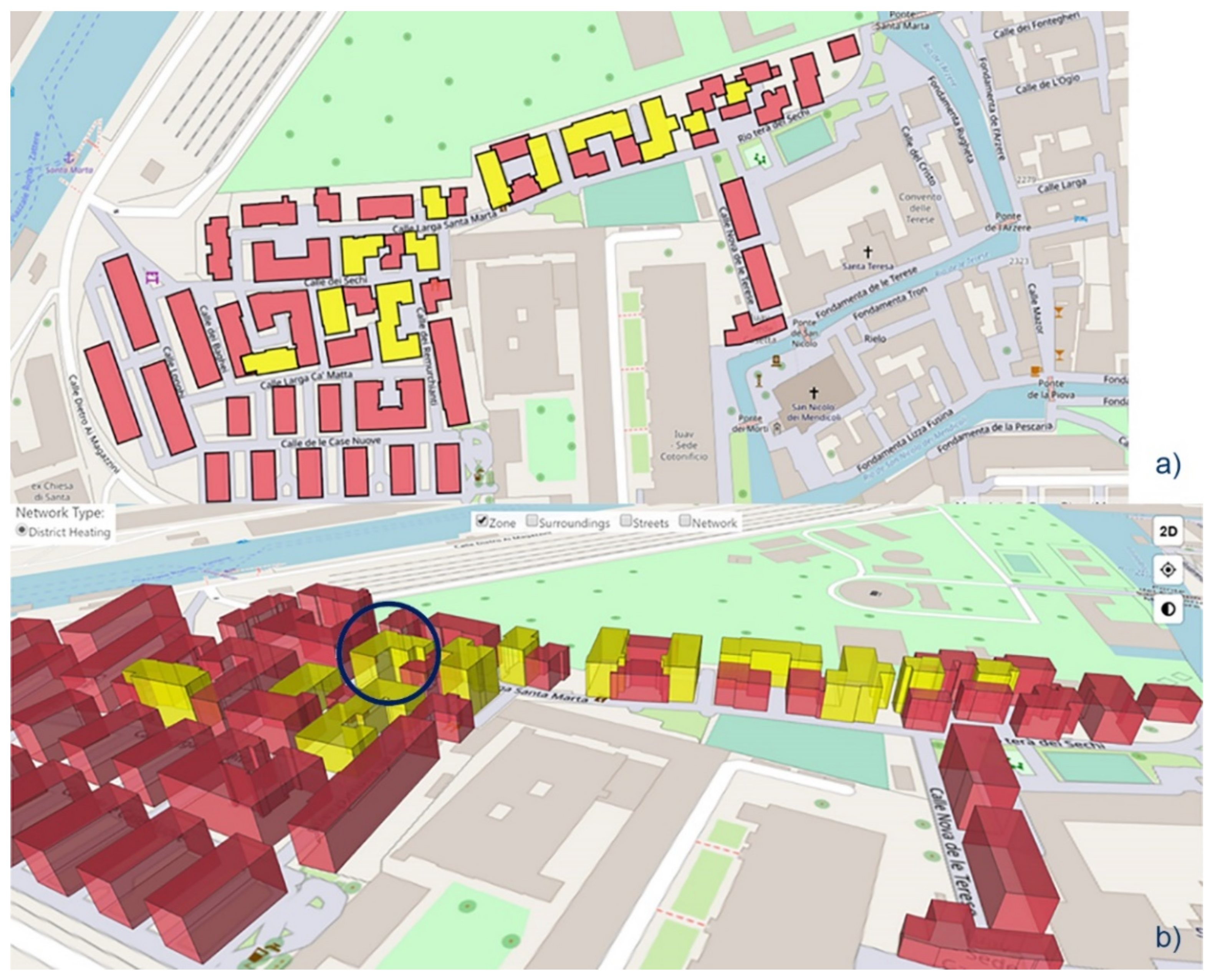
3. Case Study
4. Computer Simulations
4.1. Weather Data
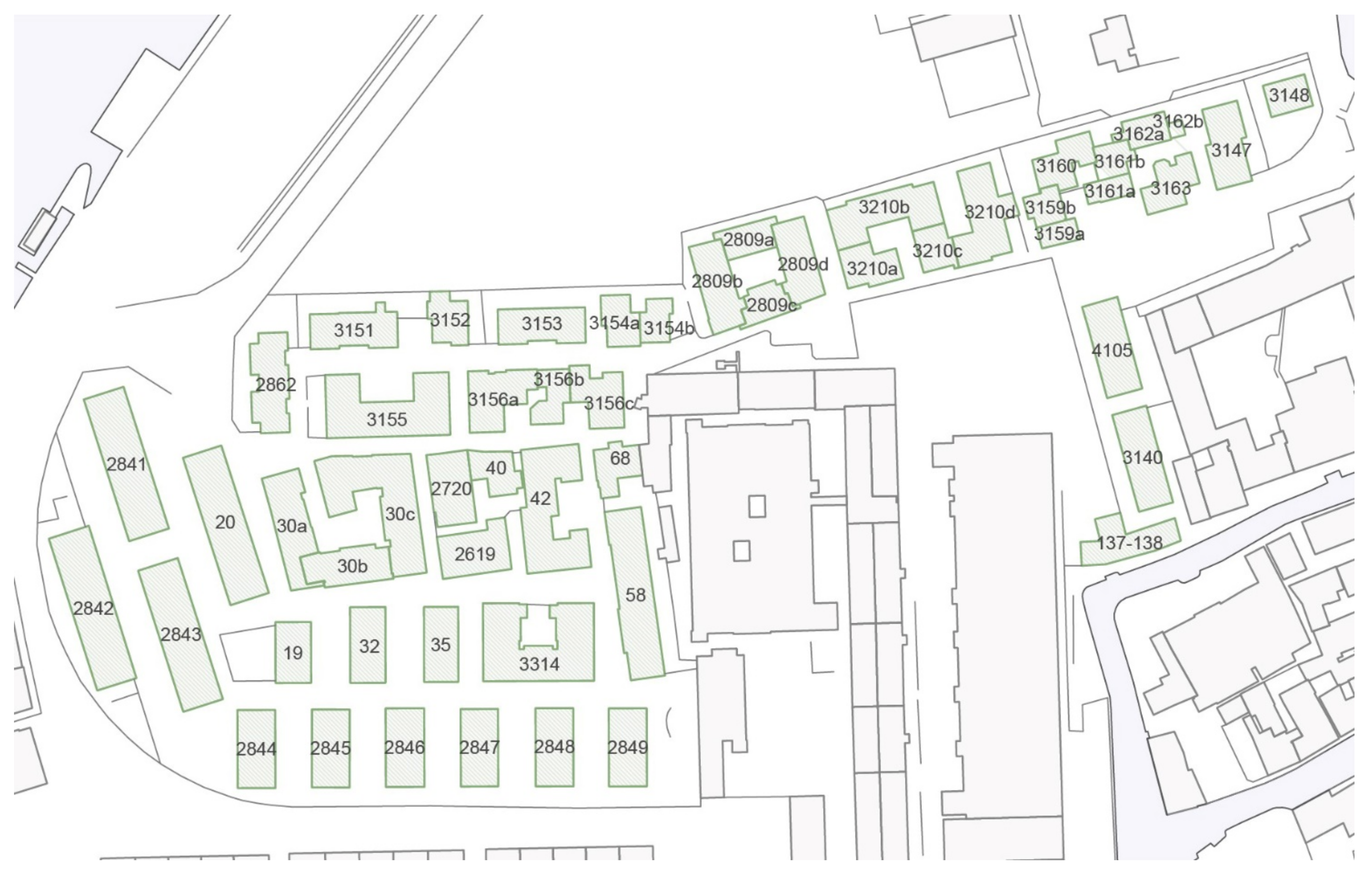
4.2. Geometry
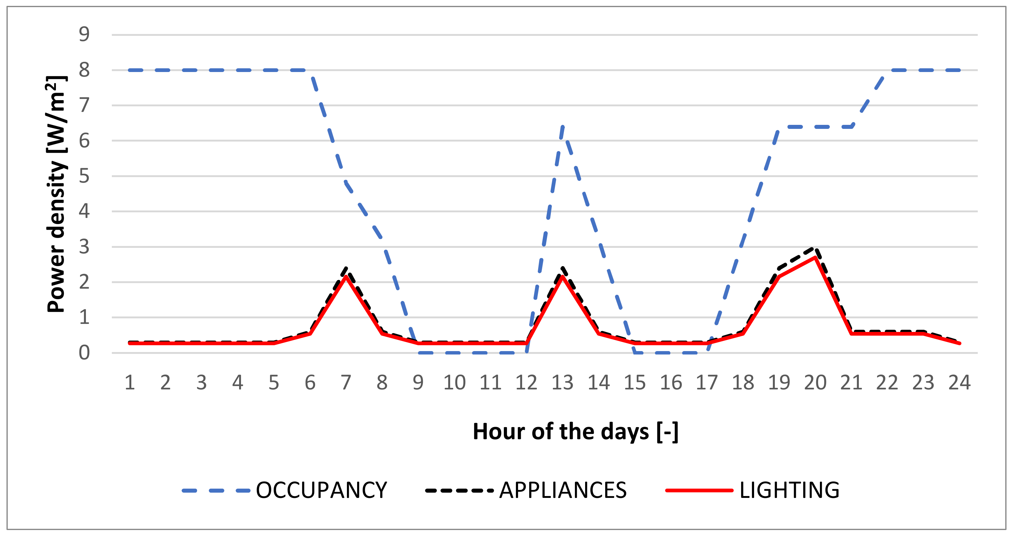
4.3. Internal Gains
4.4. Solar Gains
5. Results
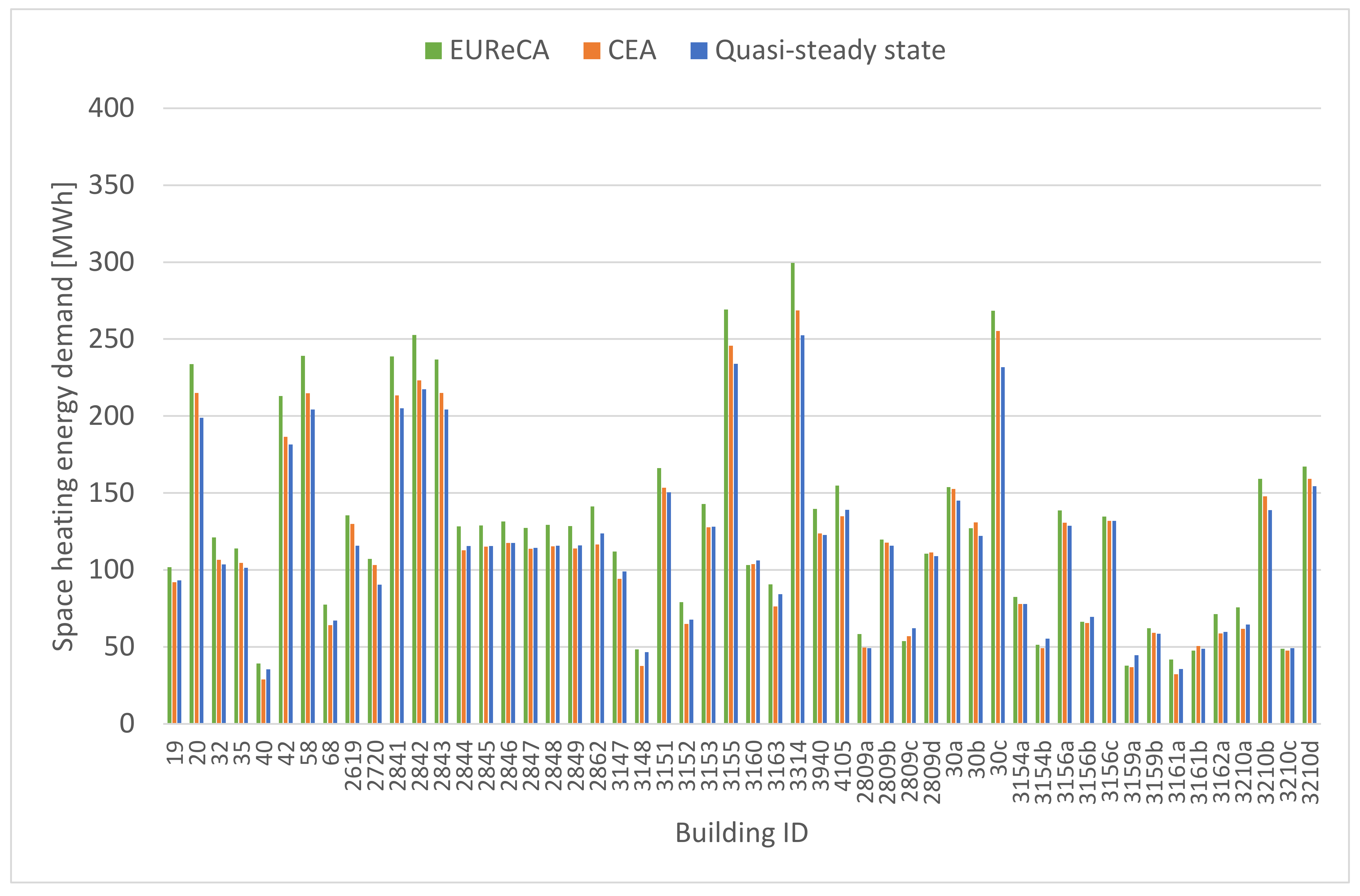
- S01—Infiltration rate and internal gains neglected, to consider only the influence of the envelope transmission losses;
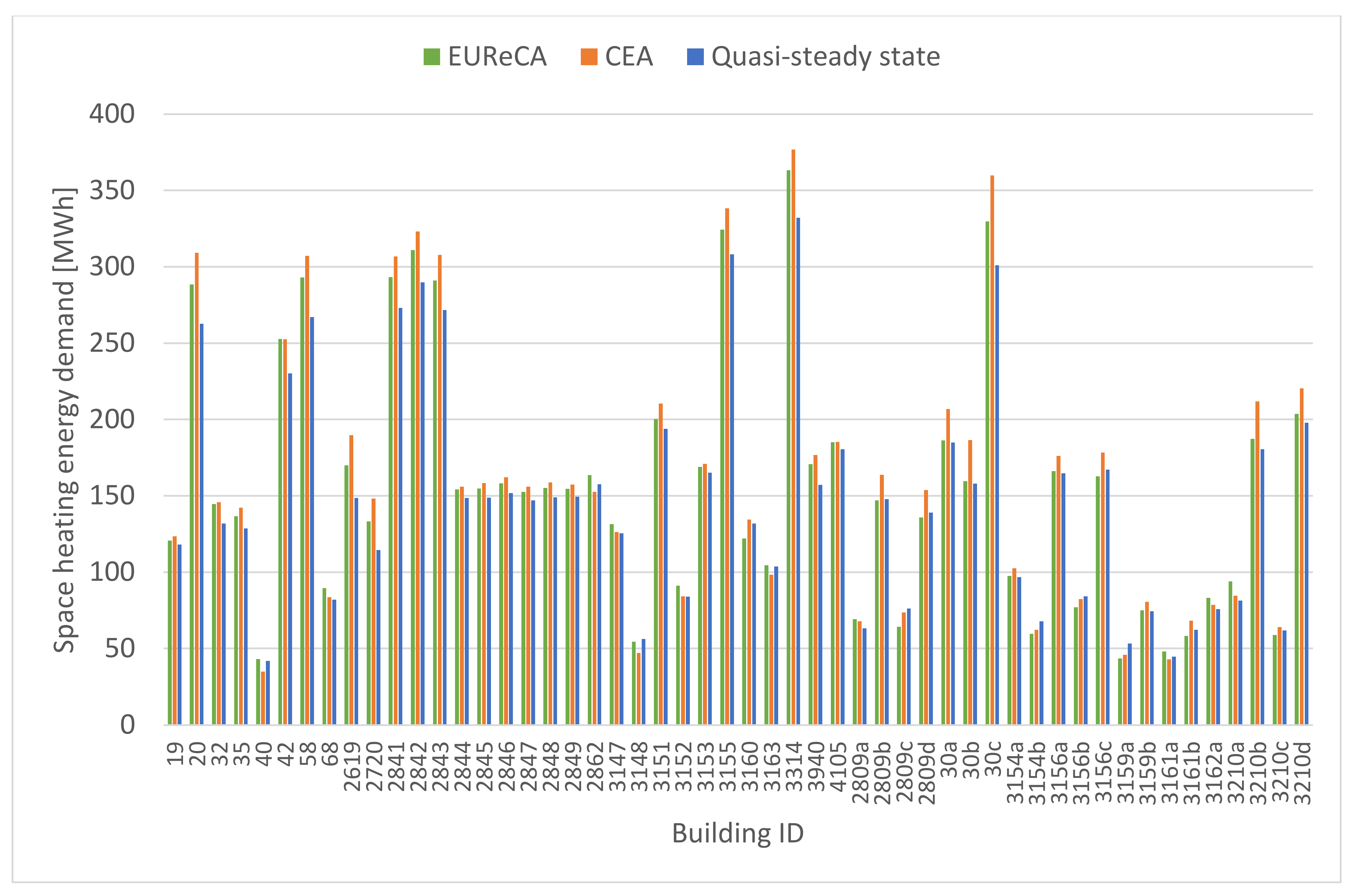
- S02—Evaluation of the infiltration rate set equal to 0.5 h−1;
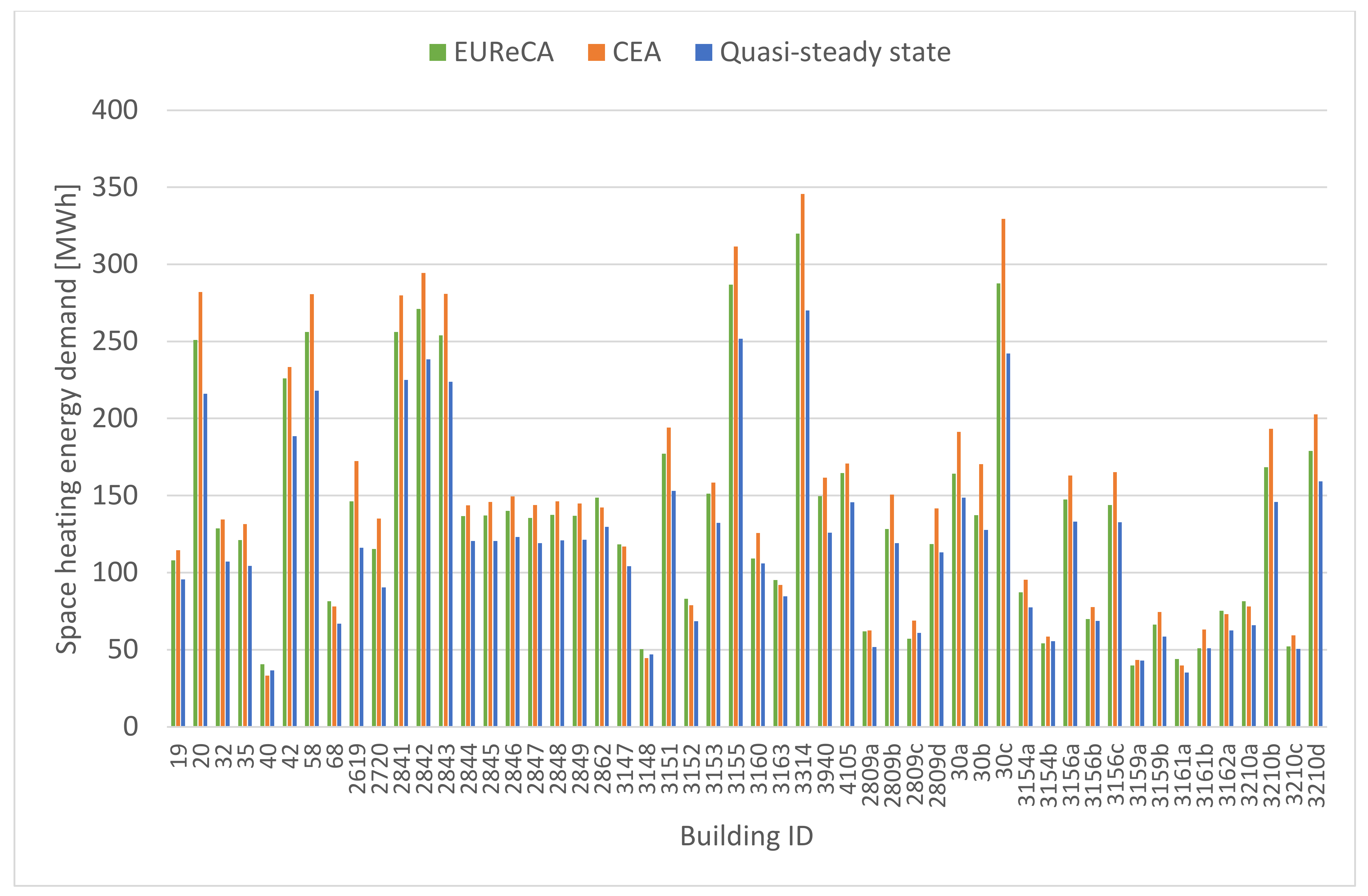
- S03—Calculation of the heating energy demand considering both internal heat gains and infiltration.
5.1. Case S01
5.2. Case S02
5.3. Case S03
5.4. Discussion
6. Conclusions
Author Contributions
Funding
Institutional Review Board Statement
Informed Consent Statement
Data Availability Statement
Conflicts of Interest
References
- Tukker, A.; Huppes, G.; Guinée, J.; Heijungs, R.; de Koning, A.; van Oers, L.; Suh, S.; Geerken, T.; van Holderbeke, M.; Jansen, B.; et al. Environmental impact of products (EIPRO). Eur. Comm. Jt. Res. Cent. 2006, 303–308. [Google Scholar]
- Eurostat Energy Database. Transport and Environment Indicators; Publications Office of the European Union: Luxembourg, 2018. [Google Scholar] [CrossRef]
- Masha, R.T.; Houreld, N.N.; Abrahamse, H. Low-Intensity Laser Irradiation at 660 nm Stimulates Transcription of Genes Involved in the Electron Transport Chain. Photomed. Laser Surg. 2013, 31, 47–53. [Google Scholar] [CrossRef]
- European Commission. EU Energy in Figures—Statistical Pocketbook; Publications Office of the European Union: Luxembourg, 2009. [Google Scholar] [CrossRef]
- Balaras, C.A.; Droutsa, K.; Dascalaki, E.; Kontoyiannidis, S. Service life of building elements & installations in European apartment buildings. In Proceedings of the 10DBMC International Conférence on Durability of Building Materials and Components, Lyon, France, 17–20 April 2005. [Google Scholar] [CrossRef]
- Piccardo, C.; Dodoo, A.; Gustavsson, L.; Tettey, U. Retrofitting with different building materials: Life-cycle primary energy implications. Energy 2019, 192, 116648. [Google Scholar] [CrossRef]
- Mastrucci, A.; Marvuglia, A.; Benetto, E.; Leopold, U. A spatio-temporal life cycle assessment framework for building renovation scenarios at the urban scale. Renew. Sustain. Energy Rev. 2020, 126, 109834. [Google Scholar] [CrossRef] [Green Version]
- ISTAT. Dati Censimento Della Popolazione. 2014. Available online: http://dati-censimentopopolazione.istat.it/ (accessed on 5 May 2021).
- ENEA. Energy Efficiency Trends and Policies in Italy; ENEA: Rome, Italy, 2018; pp. 1–37. [Google Scholar]
- Bianco, V.; Scarpa, F.; Tagliafico, L.A. Analysis and future outlook of natural gas consumption in the Italian residential sector. Energy Convers. Manag. 2014, 87, 754–764. [Google Scholar] [CrossRef]
- Toosi, H.A.; Lavagna, M.; Leonforte, F.; Del Pero, C.; Aste, N. Life Cycle Sustainability Assessment in Building Energy Retrofitting; A Review. Sustain. Cities Soc. 2020, 60, 102248. [Google Scholar] [CrossRef]
- Su, S.; Li, X.; Zhu, Y. Dynamic assessment elements and their prospective solutions in dynamic life cycle assessment of buildings. Build. Environ. 2019, 158, 248–259. [Google Scholar] [CrossRef]
- The European Parliament and the Council of the European Union. Directive 2010/31/EC of the European Parliament and of the Council of 19 May 2010 on the Energy Performance of Buildings, Official Journal of the European Union L315/1, Brussels, Belgium. 2010. Available online: https://eur-lex.europa.eu/legal-content/IT/ALL/?uri=celex:32010L0031 (accessed on 5 May 2021).
- Paiho, S.; Ketomäki, J.; Kannari, L.; Häkkinen, T.; Shemeikka, J. A new procedure for assessing the energy-efficient refurbishment of buildings on district scale. Sustain. Cities Soc. 2019, 46, 101454. [Google Scholar] [CrossRef]
- Doyle, M.D. Investigation of Dynamic and Steady State Calculation Methodologies for Determination of Building Energy Performance in the Context of the EPBD, Engineering. Ph.D. Thesis, Technological University Dublin, Dublin, Ireland, 2008. [Google Scholar] [CrossRef]
- Kim, S.H. Selection of Energy Conservation Measures for Building Energy Retrofit: A Comparison between Quasi-steady State and Dynamic Simulations in the Hands of Users. KIEAE J. 2016, 16, 5–12. [Google Scholar] [CrossRef] [Green Version]
- Corrado, V.; Fabrizio, E. Steady-State and Dynamic Codes, Critical Review, Advantages and Disadvantages, Accuracy, and Reliability. In Handbook of Energy Efficiency in Buildings; Butterworth-Heinemann: Oxford, UK, 2019; pp. 263–294. [Google Scholar] [CrossRef]
- Castaldo, V.L.; Pisello, A.L. Uses of dynamic simulation to predict thermal-energy performance of buildings and districts: A review. Wiley Interdiscip. Rev. Energy Environ. 2017, 7, e269. [Google Scholar] [CrossRef]
- Zakula, T.; Bagaric, M.; Ferdelji, N.; Milovanovic, B.; Mudrinic, S.; Ritosa, K. Comparison of dynamic simulations and the ISO 52016 standard for the assessment of building energy performance. Appl. Energy 2019, 254, 113553. [Google Scholar] [CrossRef]
- Connolly, D.; Lund, H.; Mathiesen, B.; Leahy, M. A review of computer tools for analysing the integration of renewable energy into various energy systems. Appl. Energy 2010, 87, 1059–1082. [Google Scholar] [CrossRef]
- Crawley, D.B.; Lawrie, L.K.; Winkelmann, F.C.; Buhl, W.; Huang, Y.; Pedersen, C.O.; Strand, R.K.; Liesen, R.J.; Fisher, D.E.; Witte, M.J.; et al. EnergyPlus: Creating a new-generation building energy simulation program. Energy Build. 2001, 33, 319–331. [Google Scholar] [CrossRef]
- Ratnasari, L.D.; Sangadji, S.T.M.T.S.; Safitri, S.T.M.T.E. Evaluation of energy consumption with energyplus simulation in office existing buildings. AIP Conf. Proc. 2020, 2296, 020031. [Google Scholar] [CrossRef]
- Lee, S.W.; Qian, X.; Garcia, S. An analysis of integrated ventilation systems with desiccant wheels for energy conservation and IAQ improvement in commercial buildings. Int. J. Bio-Urban. 2013, 105–124. Available online: https://scholar.google.com/citations?view_op=view_citation&hl=en&user=MnB9KIAAAAAJ&citation_for_view=MnB9KIAAAAAJ:u-x6o8ySG0sC (accessed on 15 July 2021).
- Rhodes, J.D.; Gorman, W.H.; Upshaw, C.R.; Webber, M.E. Using BEopt (EnergyPlus) with energy audits and surveys to predict actual residential energy usage. Energy Build. 2015, 86, 808–816. [Google Scholar] [CrossRef] [Green Version]
- Ligade, J.; Sebastian, D.; Razban, A. Challenges of creating a verifiable building energy model. ASHRAE Trans. 2019, 125, 20–28. [Google Scholar]
- Qian, X.; Lee, S.W. The Design and Analysis of Energy Efficient Building Envelopes for the Commercial Buildings by Mixed-levelFactorial Design and Statistical Methods. In Proceedings of the ASEE Middle Atlantic American Society of Engineering Education, Swarthmore, PA, USA, 14–15 November 2014. [Google Scholar]
- Sartor, K.; Quoilin, S.; Dewallef, P. Simulation and optimization of a CHP biomass plant and district heating network. Appl. Energy 2014, 130, 474–483. [Google Scholar] [CrossRef] [Green Version]
- Frayssinet, L.; Merlier, L.; Kuznik, F.; Hubert, J.-L.; Milliez, M.; Roux, J.-J. Modeling the heating and cooling energy demand of urban buildings at city scale. Renew. Sustain. Energy Rev. 2018, 81, 2318–2327. [Google Scholar] [CrossRef] [Green Version]
- Happle, G.; Fonseca, J.A.; Schlueter, A. A review on occupant behavior in urban building energy models. Energy Build. 2018, 174, 276–292. [Google Scholar] [CrossRef] [Green Version]
- Mosteiro-Romero, M.; Hischier, I.; Fonseca, J.A.; Schlueter, A. A novel population-based occupancy modeling approach for district-scale simulations compared to standard-based methods. Build. Environ. 2020, 181, 107084. [Google Scholar] [CrossRef]
- Bollinger, L.A.; Evins, R. HUES: A holistic urban energy simulation platform for effective model integration. In Proceedings of the International Conference CISBAT 2015 Future Buildings and Districts Sustainability from Nano to Urban Scale, Lausanne, Switzerland, 9–11 September 2015; pp. 841–846. [Google Scholar]
- Allegrini, J.; Orehounig, K.; Mavromatidis, G.; Ruesch, F.; Dorer, V.; Evins, R. A review of modelling approaches and tools for the simulation of district-scale energy systems. Renew. Sustain. Energy Rev. 2015, 52, 1391–1404. [Google Scholar] [CrossRef]
- Keirstead, J.; Jennings, M.; Sivakumar, A. A review of urban energy system models: Approaches, challenges and opportunities. Renew. Sustain. Energy Rev. 2012, 16, 3847–3866. [Google Scholar] [CrossRef] [Green Version]
- Bourdic, L.; Salat, S. Building energy models and assessment systems at the district and city scales: A review. Build. Res. Inf. 2012, 40, 518–526. [Google Scholar] [CrossRef]
- Plan4DE. Available online: http://plan4de.ssg.coop/ (accessed on 8 July 2021).
- EXCEED. Available online: https://dashboard.exceedproject.eu/ (accessed on 8 July 2021).
- Toolbox. Available online: https://www.hotmaps.eu/map (accessed on 8 July 2021).
- Zhang, X.; Strbac, G.; Shah, N.; Teng, F.; Pudjianto, D. Whole-System Assessment of the Benefits of Integrated Electricity and Heat System. IEEE Trans. Smart Grid 2018, 10, 1132–1145. [Google Scholar] [CrossRef]
- Fonseca, J.A. Energy Efficiency Strategies in Urban Communities: Modeling, Analysis and Assessment. Ph.D. Thesis, ETH Zurich, Zurich, Switzerland, 2016. [Google Scholar] [CrossRef]
- Fonseca, J.A.; Thomas, D.; Willmann, A.; Elesawy, A.; Schlueter, A. The City Energy Analyst Toolbox V0.1. In Proceedings of the Sustainable Built Environment (SBE) Regional Conference, Zurich, Switzerland, 15–17 June 2006. [Google Scholar] [CrossRef]
- Romano, P.; Prataviera, E.; Carnieletto, L.; Vivian, J.; Zinzi, M.; Zarrella, A. Assessment of the Urban Heat Island Impact on Building Energy Performance at District Level with the EUReCA Platform. Climate 2021, 9, 48. [Google Scholar] [CrossRef]
- Prataviera, E.; Romano, P.; Carnieletto, L.; Pirotti, F.; Vivian, J.; Zarrella, A. EUReCA: An open-source urban building energy modelling tool for the efficient evaluation of cities energy demand. Renew. Energy 2021, 173, 544–560. [Google Scholar] [CrossRef]
- Vivian, J.; Zarrella, A.; Emmi, G.; De Carli, M. An evaluation of the suitability of lumped-capacitance models in calculating energy needs and thermal behaviour of buildings. Energy Build. 2017, 150, 447–465. [Google Scholar] [CrossRef]
- Comité Europeo de Normalización. ISO 13790:2008 Energy Performance of Buildings: Calculation of Energy Use for Space Heating and Cooling (ISO 13790:2008); CEN: Brusseles, Switzerland, 2008. [Google Scholar]
- Fonseca, J.A.; Schlueter, A. Integrated model for characterization of spatiotemporal building energy consumption patterns in neighborhoods and city districts. Appl. Energy 2015, 142, 247–265. [Google Scholar] [CrossRef]
- Fonseca, J.A.; Nguyen, T.-A.; Schlueter, A.; Marechal, F. City Energy Analyst (CEA): Integrated framework for analysis and optimization of building energy systems in neighborhoods and city districts. Energy Build. 2016, 113, 202–226. [Google Scholar] [CrossRef]
- Zarrella, A.; Prataviera, E.; Romano, P.; Carnieletto, L.; Vivian, J. Analysis and application of a lumped-capacitance model for urban building energy modelling. Sustain. Cities Soc. 2020, 63, 102450. [Google Scholar] [CrossRef]
- Weather Data|EnergyPlus. Available online: https://www.energyplus.net/weather (accessed on 18 March 2021).
- Ente Nazionale Italiano di Unificazione. UNI/TS 11300—Part 1: Evaluation of Energy Need for Space Heating and Cooling; UNI: Milan, Italy, 2014. [Google Scholar]
- Mora, T.D.; Peron, F.; Romagnoni, P.; Almeida, M.; Ferreira, M. Tools and procedures to support decision making for cost-effective energy and carbon emissions optimization in building renovation. Energy Build. 2018, 167, 200–215. [Google Scholar] [CrossRef]
- Thomsen, K.E.; Rose, J.; Mørck, O.; Jensen, S.; Østergaard, I.; Knudsen, H.N.; Bergsøe, N.C. Energy consumption and indoor climate in a residential building before and after comprehensive energy retrofitting. Energy Build. 2016, 123, 8–16. [Google Scholar] [CrossRef]
- Ministro della Salute, Ministro dell’Ambiente, Ministro delle Infrastrutture, Decreto Ministeriale 26 August 2015, Applicazione Delle Metodologie di Calcolo Delle Prestazioni Energetiche e defi Nizione delle Prescrizioni e dei Requisiti Minimi Degli Edifici. 2015. Available online: https://www.gazzettaufficiale.it/eli/gu/2015/07/15/162/so/39/sg/pdf (accessed on 5 May 2021).
- Comitato Termotecnico Italiano CTI, Archivi Anni Tipo Climatici. 2015. Available online: https://shop.cti2000.it/ (accessed on 5 May 2021).
- CEN (European Committee for Standardization). EN ISO 15927-4: 2005--Hygrothermal Performance of Buildings--Calculation and Presentation of Climatic Data--Part 4: Hourly Data for Assessing the Annual Energy Use for Heating and Cooling; CEN: Brusseles, Switzerland, 2005. [Google Scholar]
- Italian Organisation for Stardardisation (UNI). UNI 10349-1:2016, Heating and Cooling of Buildings—Climatic Data—Part 1: Monthly Means for Evaluation of Energy Need for Space Heating and Cooling and Methods for Splitting Global Solar Irradiance into the Direct and Diffuse Parts and for Calculate; CEN: Brusseles, Switzerland, 2016. [Google Scholar]
- Decreto del Presidente della Repubblica. Decreto del Presidente della Repubblica n. 412 del 26 agosto 1993, “Regolamento Recante Norme per la Progettazione, l’installazione, l’esercizio e la Manutenzione Degli Impianti Termici Degli Edifici ai Fini del Contenimento dei Consumi di Energia, in att; CEN: Brusseles, Switzerland, 1993. [Google Scholar]
- Il Presidente della Repubblica. Italian Law n.74/2013, Gazz. Uff. 27 Giugno 2013, n. 149. 2013, pp. 1–11. Available online: http://www.energia.provincia.tn.it/binary/pat_agenzia_energia/dpr74-2013.pdf (accessed on 5 May 2021).
- UNI Ente Nazionale Italiano di Unificazione. UNI/TS 11300; UNI Ente Nazionale Italiano di Unificazione: Milano, Italy, 2008. [Google Scholar]
- Legge 31 Maggio 1903, n. 254, “Sulle case popolari,” Gazz. Uff. (1903). Available online: https://www.gazzettaufficiale.it/atto/serie_generale/caricaDettaglioAtto/originario?atto.dataPubblicazioneGazzetta=1903-07-08&atto.codiceRedazionale=003U0254 (accessed on 19 February 2020).
- L’ATER di Venezia e la sua Storia|ATER Venezi. Available online: https://web.archive.org/web/20150114032956/http://www.atervenezia.it/informazioni-generali/la-storia-il-profilo-operativo-e-le-cifre-dellente/later-di-venezia-e-la-sua-storia/ (accessed on 19 February 2020).
- Azienda Territoriale per l’Edilizia Residenziale L’ATER di Venezia e la sua Storia. Available online: https://www.atervenezia.it/ente/later-di-venezia-e-la-sua-storia/ (accessed on 19 February 2020).
- Case Dello IACP a Santa Marta, già Quartieri “Benito Mussolini” e “SADE”|Conoscere Venezia. Available online: https://www.conoscerevenezia.it/?p=43647 (accessed on 19 February 2020).
- Venice EPW Weather Data. Available online: https://energyplus.net/weather-location/europe_wmo_region_6/ITA//ITA_Venezia-Tessera.161050_IGDG (accessed on 19 February 2020).
- Murano, G.; Corrado, V.; Dirutigliano, D. The new Italian Climatic Data and their Effect in the Calculation of the Energy Performance of Buildings. Energy Procedia 2016, 101, 153–160. [Google Scholar] [CrossRef] [Green Version]
- CEN (European Committee for Standardization). EN ISO 15927-6:2007 Hygrothermal Performance of Buildings—Calculation and Presentation of Climatic Data—Part 6: Accumulated Temperature Differences (Degree-Days); CEN: Brusseles, Switzerland, 2007; pp. 1–13. [Google Scholar]
- Quantum GIS. Available online: https://www.qgis.org/en/site/ (accessed on 28 January 2021).
- Open Street Map. Available online: https://www.openstreetmap.org/ (accessed on 28 January 2021).
- Mutani, G.; Vicentini, G. Analisi del fabbisogno di energia termica degli edifici con software geografico libero. Il caso studio di Torino. La Termotec. 2013, 6, 63–67. [Google Scholar]
- Agugiaro, G. Energy planning tools and CityGML-based 3D virtual city models: Experiences from Trento (Italy). Appl. Geomat. 2015, 8, 41–56. [Google Scholar] [CrossRef]
- Google Maps. Available online: https://www.google.com/maps/@45.4387765,12.3380271,13.26z?hl=en-GB&authuser=0 (accessed on 27 February 2020).
- Bing Maps—Directions, Trip Planning, Traffic Cameras & More. Available online: https://www.bing.com/maps (accessed on 27 February 2020).
- Barbiani, E. Edilizia Popolare a Venezia; Mondadori Electa: Milano, Italy, 1983. [Google Scholar]
- European Committee for Standardization-CEN. BS EN 16798—Energy Performance of Buildings—Ventilation for Buildings—Part 1: Indoor Environmental Input Parameters For Design And Assessment of Energy Performance Of Buildings Addressing Indoor Air Quality, Thermal Environment, Lighting And Acoustic; CEN: Brussels, Belgium, 2019. [Google Scholar]
- Fu, P.; Rich, P.M. A geometric solar radiation model with applications in agriculture and forestry. Comput. Electron. Agric. 2002, 37, 25–35. [Google Scholar] [CrossRef]
- Esri Support ArcMap 10.2 (10.2.1, 10.2.2). Available online: https://support.esri.com/en/products/desktop/arcgis-desktop/arcmap/10-2-2 (accessed on 8 July 2021).
- Reinhart, C.F. DAYSIM Advanced Daylight Simulation Software; MITPress: Boston, MA, USA, 2021; Available online: http://daysim.ning.com (accessed on 5 May 2021).
- Arasteh, D.; Kohler, C.; Griffith, B. Modeling Windows in Energy Plus with Simple Performance Indices; Lawrence Berkeley National Lab: Berkeley, CA, USA, 2009. [Google Scholar] [CrossRef] [Green Version]
- Cecchinato, L.; Romagnoni, P.; Schibuola, L. Building heating requirement calculation: A critical analysis of the new European standards. Int. J. Ambient. Energy 2000, 21, 21–30. [Google Scholar] [CrossRef]
- Magrini, A.; Magnani, L.; Pernetti, R. The effort to bring existing buildings towards the A class: A discussion on the application of calculation methodologies. Appl. Energy 2012, 97, 438–450. [Google Scholar] [CrossRef]
- Corrado, V.; Fabrizio, E. Il significato del fattore di utilizzazione nel calcolo semplificato del fabbisogno termico degli edifici: Aspetti teorici e applicativi. In Proceedings of the AiCARR “Certificazione Energetica: Normative e Modelli di Calcolo per il Sistema Edificio-Impianto Posti a Confronto”, Bologna, Italy, 16 October 2008. [Google Scholar]


| Element | Components from Exterior to Interior | Thermal Transmittance [W/(m2 K)] |
|---|---|---|
| External wall | External plaster (1.5 cm) Solid bricks (25 cm) Internal plaster (1.5 cm) | 1.35 |
| Floor slab | Screed (30 cm) Concrete casting (10 cm) Traditional screed (3 cm) Stoneware floor (1.5 cm) | 1.41 |
| Roof | Terracotta tiles (1.2 cm) Wood panel (3 cm) | 2.5 |
| Single-glazed windows | Wood frame Single glazing | 5.8 |
| Dry Bulb Temp—Avg Daily [°C] | Global Horiz Radiation—Avg Daily [kWh/m2] | |||
|---|---|---|---|---|
| Month\Source | Venice.epw | UNI 10349-1:2016 | Venice.epw | UNI 10349-1:2016 |
| January | 2.64 | 3.10 | 0.88 | 1.25 |
| February | 3.89 | 3.70 | 1.15 | 2.25 |
| March | 7.75 | 8.70 | 2.56 | 3.47 |
| April | 12.03 | 12.90 | 3.71 | 4.69 |
| May | 17.24 | 19.00 | 5.02 | 6.08 |
| June | 20.76 | 22.40 | 5.47 | 7.17 |
| July | 23.82 | 23.80 | 5.68 | 7.53 |
| August | 22.75 | 23.80 | 4.68 | 6.14 |
| September | 19.62 | 18.70 | 3.35 | 4.39 |
| October | 13.93 | 14.00 | 1.96 | 2.72 |
| November | 8.68 | 8.40 | 0.91 | 1.47 |
| December | 4.00 | 4.90 | 0.73 | 1.14 |
| South | East | West | North | |
|---|---|---|---|---|
| [kWh/m2] | [kWh/m2] | [kWh/m2] | [kWh/m2] | |
| January | 2.18 | 1.42 | 1.45 | 0.89 |
| February | 2.07 | 1.34 | 1.37 | 0.84 |
| March | 3.15 | 2.05 | 2.09 | 1.29 |
| April | 3.12 | 2.02 | 2.06 | 1.27 |
| October | 3.11 | 2.02 | 2.06 | 1.27 |
| November | 2.08 | 1.35 | 1.38 | 0.85 |
| December | 2.02 | 1.31 | 1.34 | 0.82 |
| Average | 2.43 | 1.58 | 1.61 | 0.99 |
| MS Excel Spreadsheet [MWh] | CEA [MWh] | EUReCA [MWh] | |
|---|---|---|---|
| S01 | 6018 | 6115 (+2%) | 6707 (+11%) (+10%) |
| S02 | 7732 | 8435 (+9%) | 8083 (+5%) (−4%) |
| S03 | 6274 | 7769 (+24%) | 7149 (+33%) (+7%) |
Publisher’s Note: MDPI stays neutral with regard to jurisdictional claims in published maps and institutional affiliations. |
© 2021 by the authors. Licensee MDPI, Basel, Switzerland. This article is an open access article distributed under the terms and conditions of the Creative Commons Attribution (CC BY) license (https://creativecommons.org/licenses/by/4.0/).
Share and Cite
Dalla Mora, T.; Teso, L.; Carnieletto, L.; Zarrella, A.; Romagnoni, P. Comparative Analysis between Dynamic and Quasi-Steady-State Methods at an Urban Scale on a Social-Housing District in Venice. Energies 2021, 14, 5164. https://doi.org/10.3390/en14165164
Dalla Mora T, Teso L, Carnieletto L, Zarrella A, Romagnoni P. Comparative Analysis between Dynamic and Quasi-Steady-State Methods at an Urban Scale on a Social-Housing District in Venice. Energies. 2021; 14(16):5164. https://doi.org/10.3390/en14165164
Chicago/Turabian StyleDalla Mora, Tiziano, Lorenzo Teso, Laura Carnieletto, Angelo Zarrella, and Piercarlo Romagnoni. 2021. "Comparative Analysis between Dynamic and Quasi-Steady-State Methods at an Urban Scale on a Social-Housing District in Venice" Energies 14, no. 16: 5164. https://doi.org/10.3390/en14165164