
An Integrated Approach for Evaluating the Restoration of the Salinity Gradient in Transitional Waters: Monitoring and Numerical Modeling in the Life Lagoon Refresh Case Study

 , , , ,
Abstract
:1. Introduction
- quantitative definition of the project objectives through numerical modeling, design of the hydraulic works and identification of the proper fresh water discharge necessary to achieve the objectives;
- implementation of the integrated analysis approach through monitoring and validated numerical modeling;
- assessment of results and verification of compliance of management objectives;
- completion of conservation actions with a step-by-step approach supported by monitoring and modeling results.
2. Materials and Methods
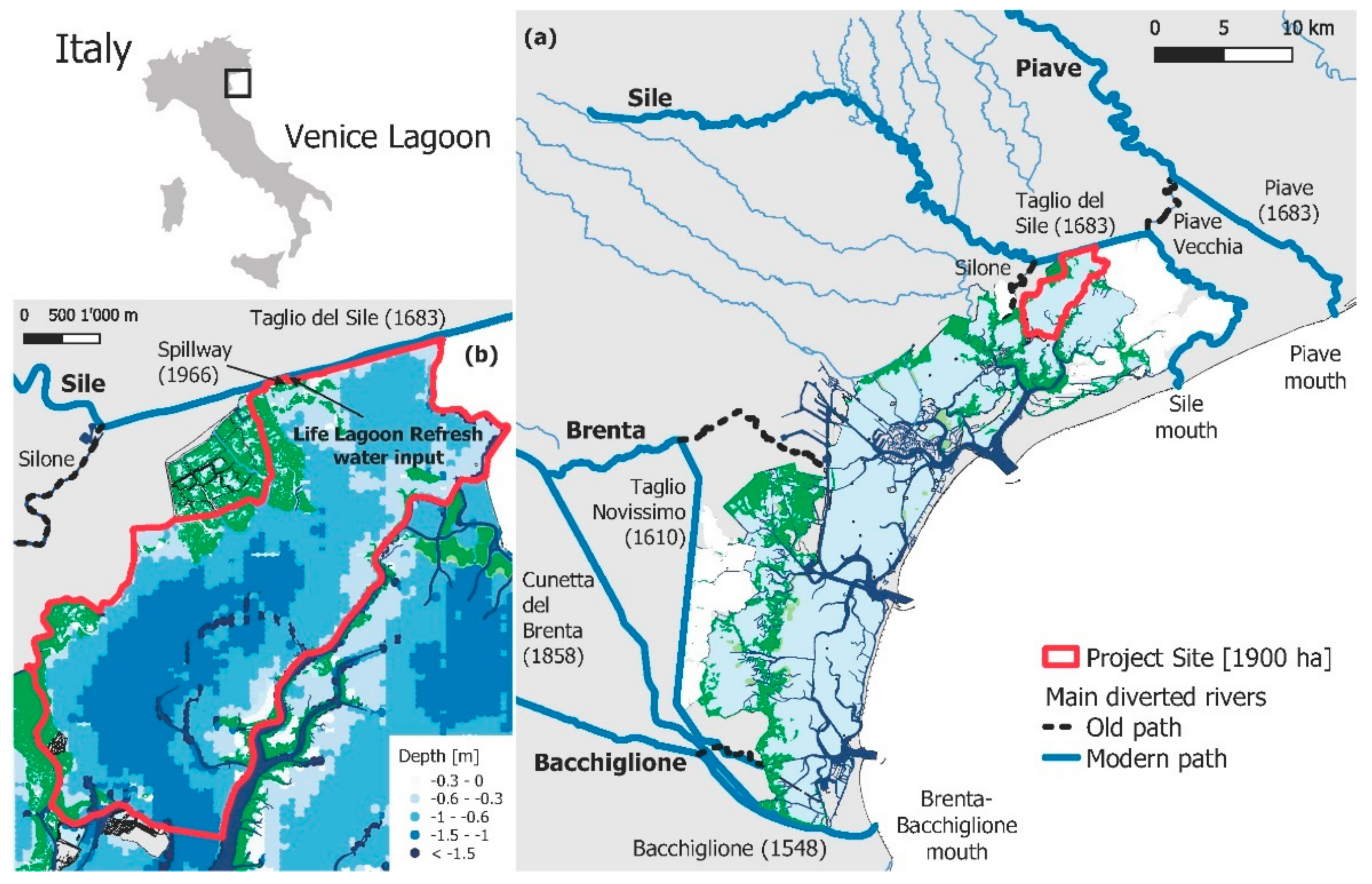
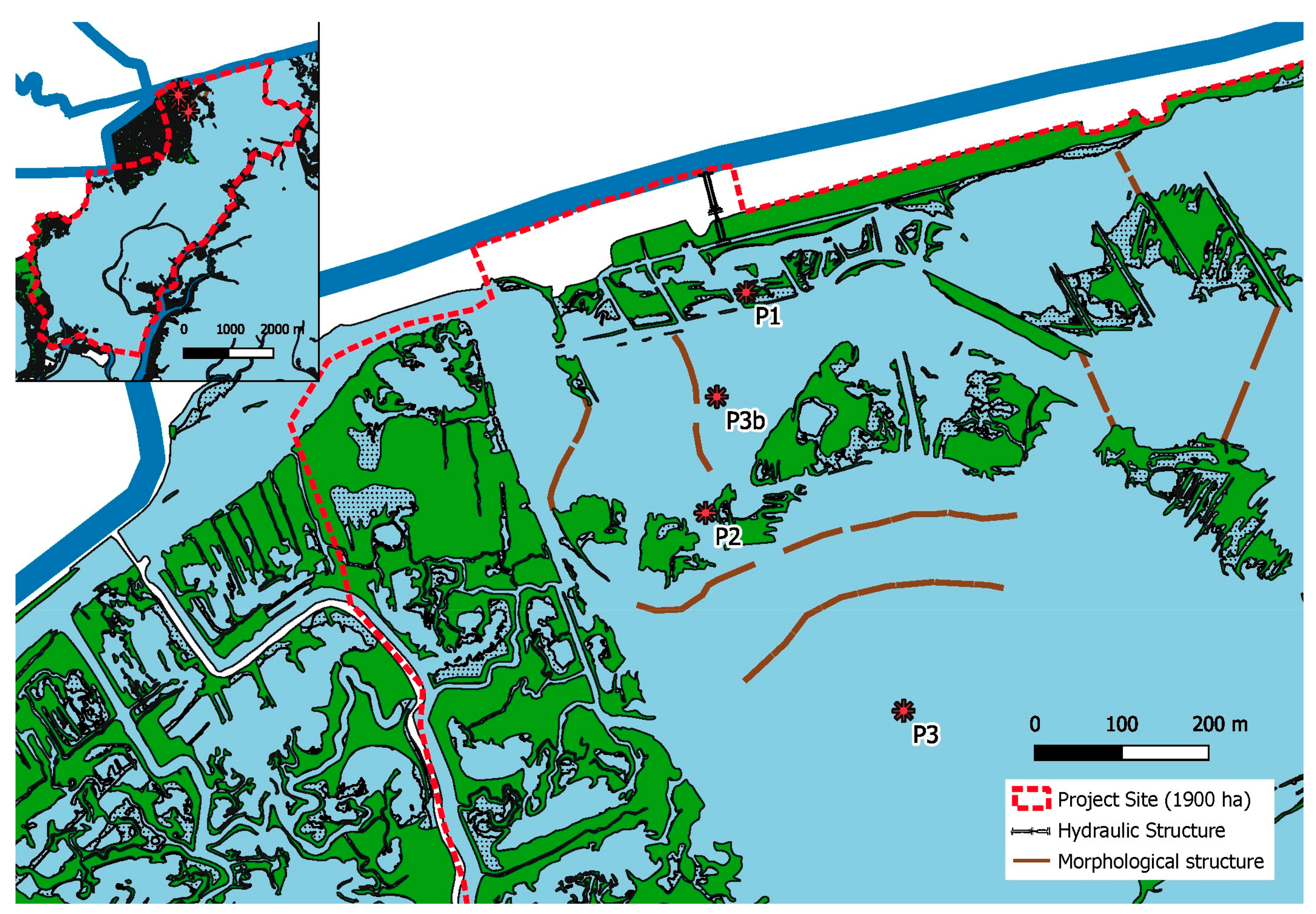
2.1. Study Area and Project Details

2.2. Moored Probes
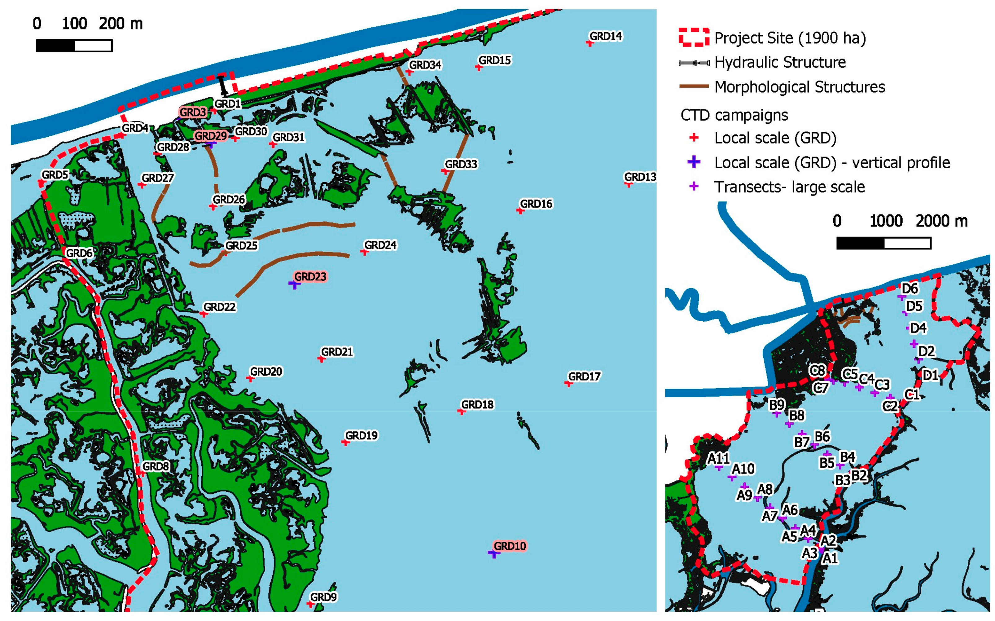
2.3. CTD Profiles
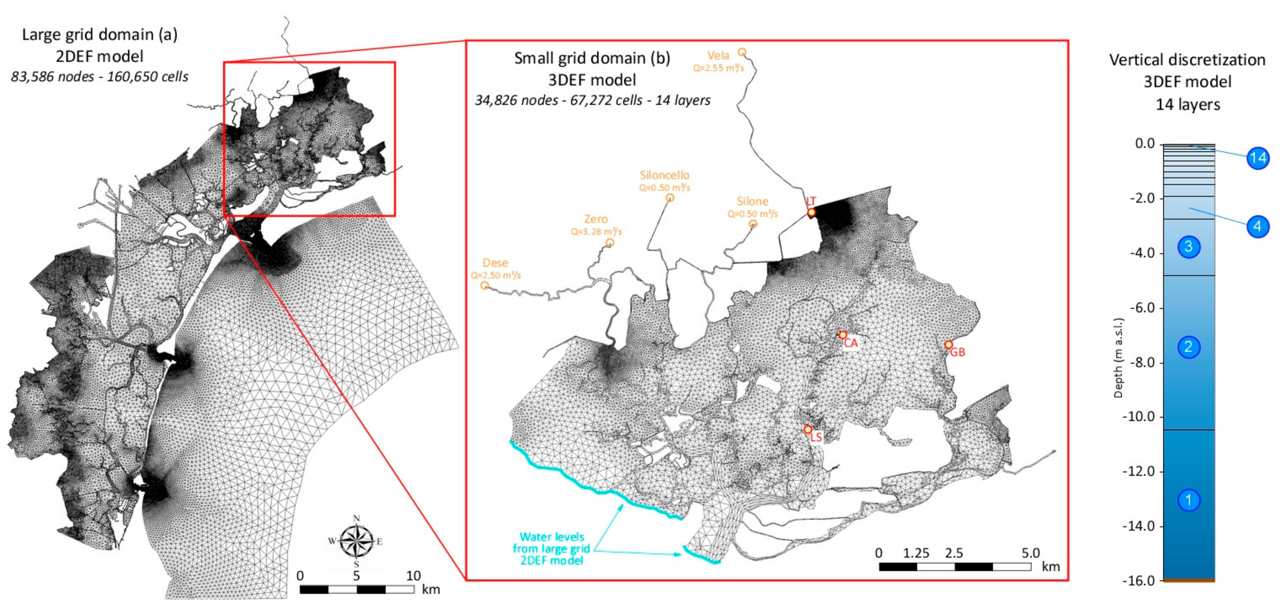
2.4. Numerical Modeling
2.5. Data Evaluation
2.5.1. Moored Probes Data
2.5.2. CTD Profile Data
2.5.3. Numerical Model Data
3. Results
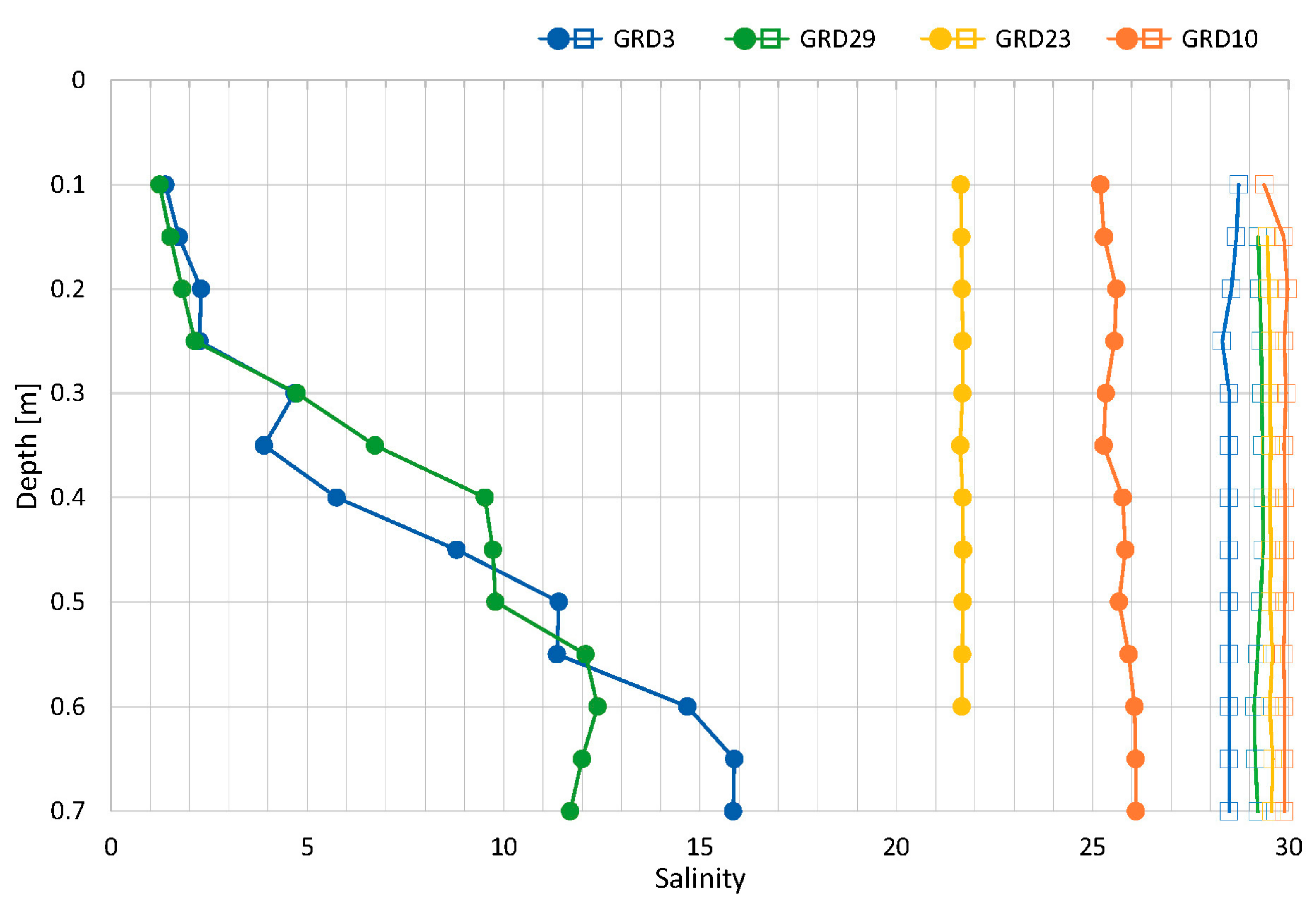
3.1. Moored Probes
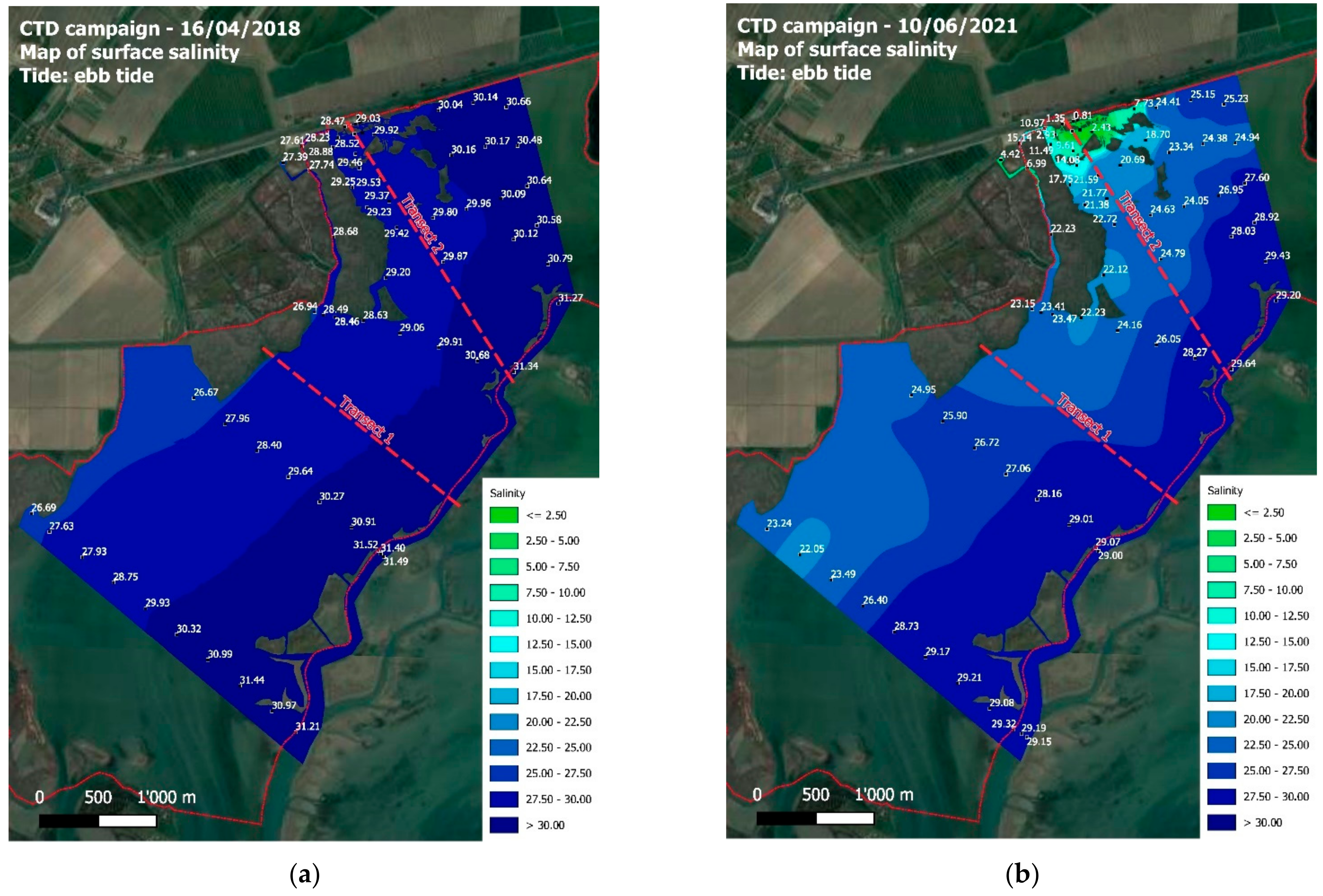
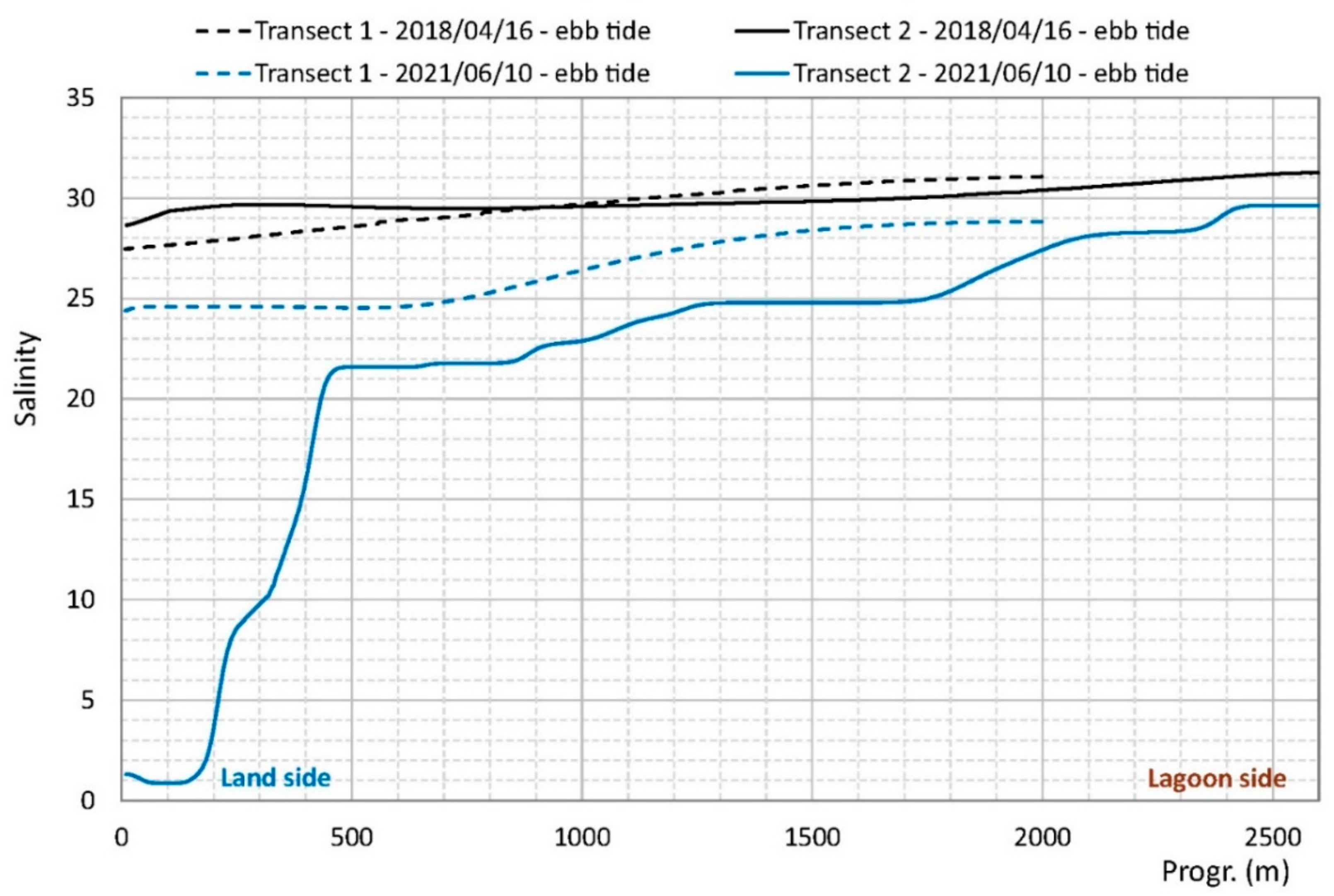
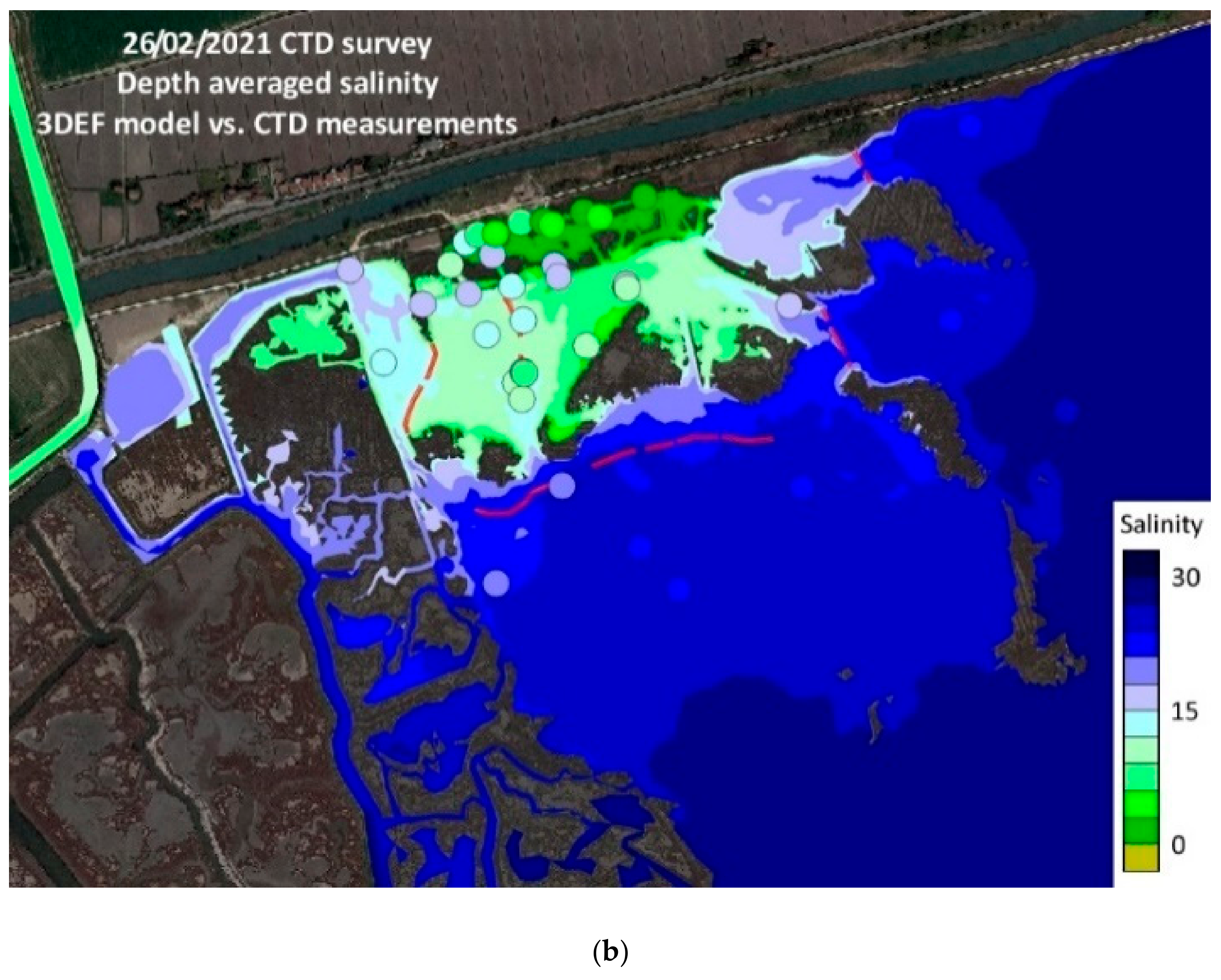
3.2. CTD Profiles
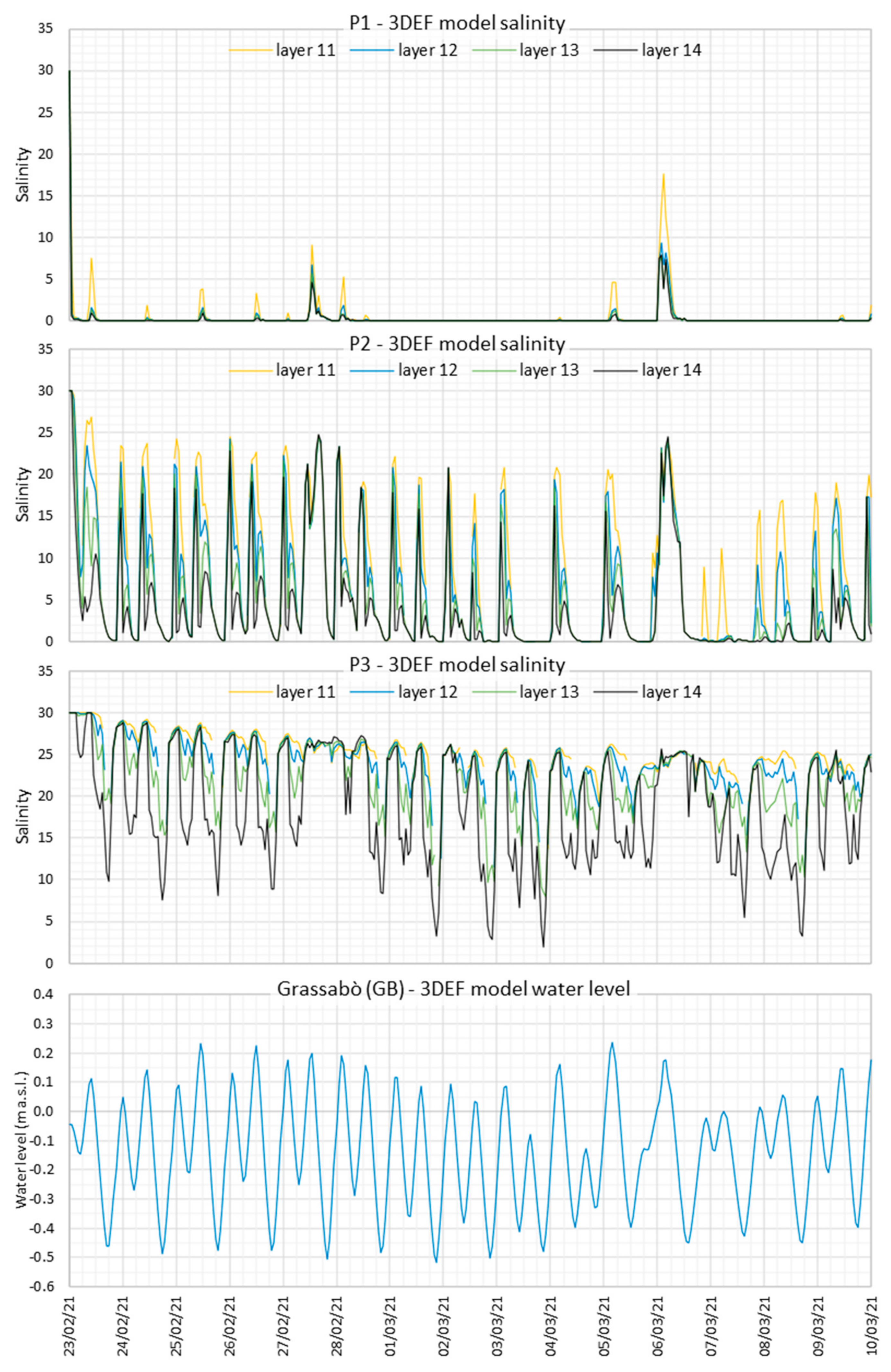
3.3. Numerical Modeling
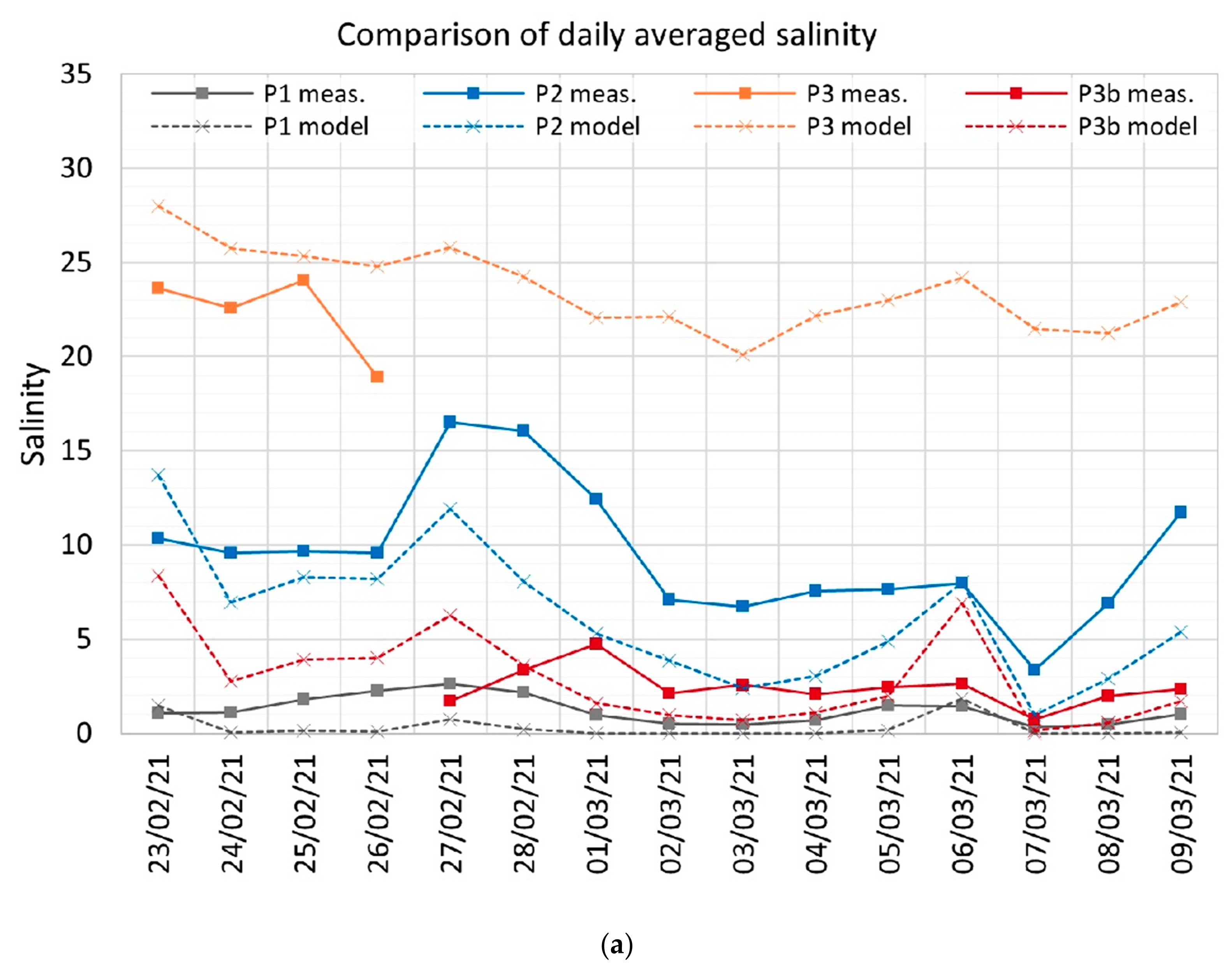
3.3.1. Model Performance
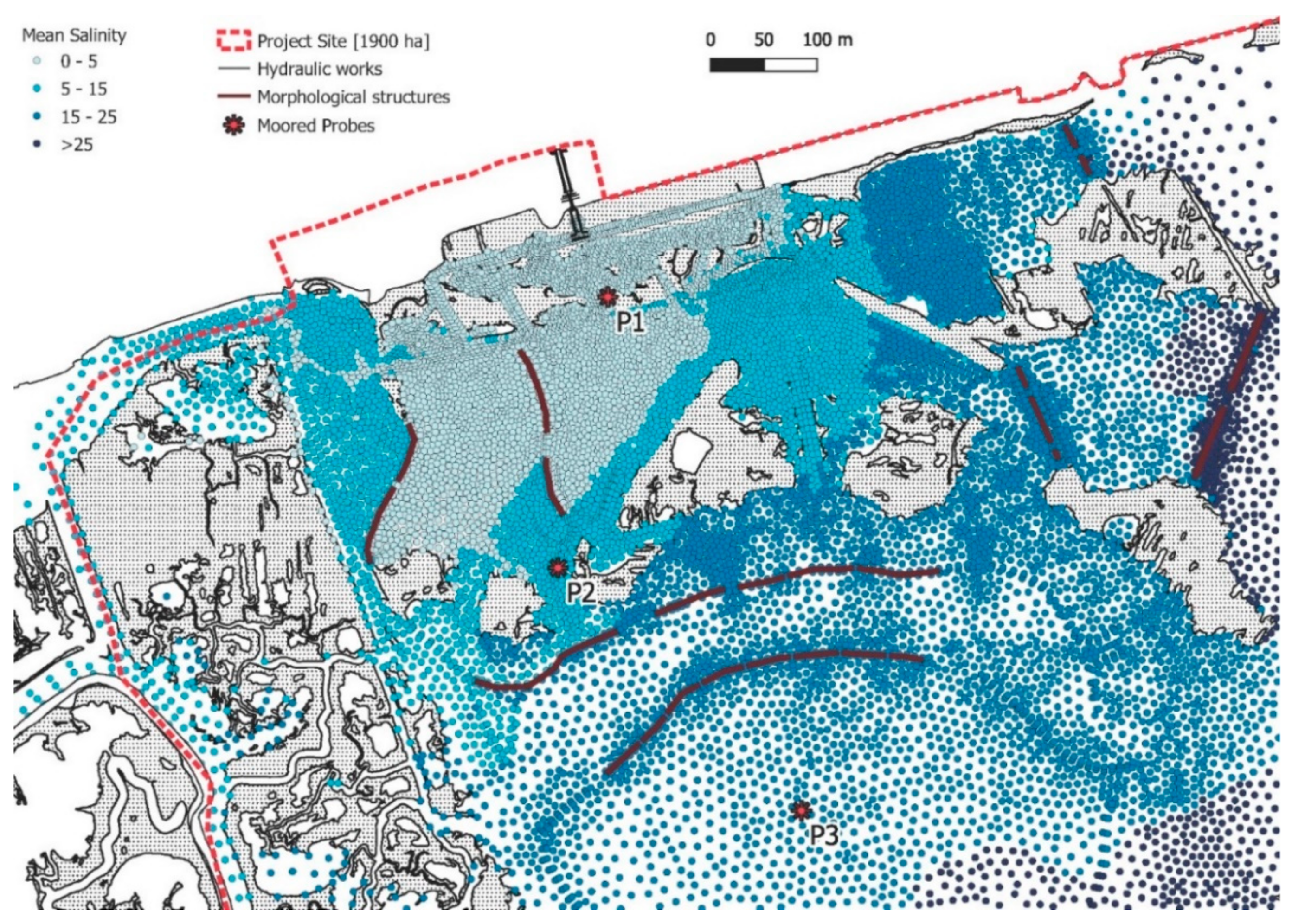
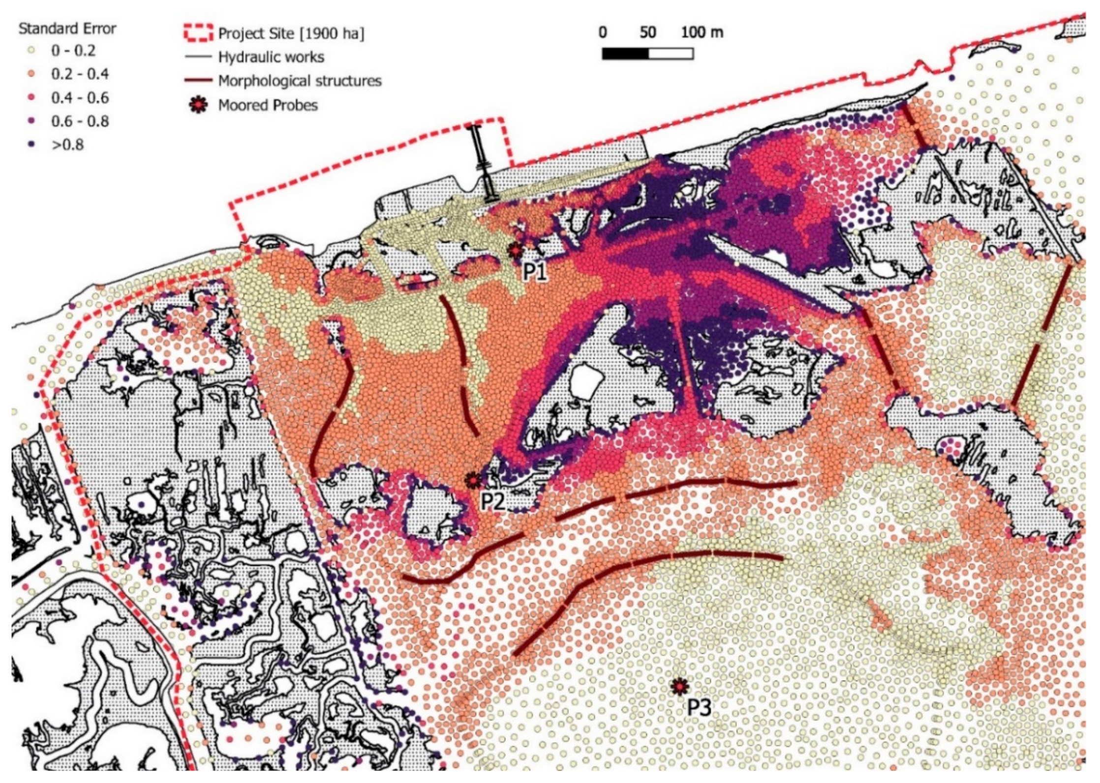
3.3.2. DrEAM Tool
4. Discussion
- the restoration of the saline gradient, main objective of the project, required a precise quantitative analysis;
- the high spatial variability, induced by the realization of the intervention with the introduction of a fresh water flow, and temporal variability on a short and medium scale, due to the interaction of the tide and the seasonal variability of the boundary conditions, required a detailed description with adequate resolution in time and space;
- each tool has different features and only an integrated approach can identify pros and cons and define a combined, effective and efficient strategy;
- the consolidated small-scale approach should be robust and applicable to all scales.
5. Conclusions
Author Contributions
Funding
Institutional Review Board Statement
Informed Consent Statement
Data Availability Statement
Conflicts of Interest
References
- Pérez-Ruzafa, A.; Marcos, C.; Pérez-Ruzafa, I. Mediterranean coastal lagoons in an ecosystem and aquatic resources management context. Phys. Chem. Earth 2011, 36, 160–166. [Google Scholar] [CrossRef]
- Cataudella, S.; Crosetti, D.; Massa, F. Mediterranean coastal lagoons: Sustainable management and interactions among aquaculture, capture fisheries and the environment. In FAO Studies and Reviews General Fisheries Commission for the Mediterranean; Food & Agriculture Organization of the United Nations (FAO): Rome, Italy, 2015; p. 293. [Google Scholar]
- Reizopoulou, S.; Simboura, N.; Barbone, E.; Aleffi, F.; Basset, A.; Nicolaidou, A. Biodiversity in transitional waters: Steeper ecotone, lower diversity. Mar. Ecol. 2014, 35, 78–84. [Google Scholar] [CrossRef]
- Tagliapietra, D.; Sigovini, M.; Volpi Ghirardini, A. A review of terms and definitions to categorize estuaries, lagoons and associated environments. Mar. Fresh Water Res. 2009, 60, 497–509. [Google Scholar] [CrossRef]
- Smyth, K.; Elliott, M. Effects of changing salinity on the ecology of the marine environment. In Stressors in the Marine Environment: Physiological and Ecological Responses; Societal Implications; Solan, M., Whiteley, N., Eds.; Oxford University Press: Oxford, UK, 2016; ISBN 13 9780198718826. [Google Scholar]
- Scapin, L.; Zucchetta, M.; Bonometto, A.; Feola, A.; Boscolo Brusà, R.; Sfriso, A.; Franzoi, P. Expected shifts in nekton community following salinity reduction: Insights into restoration and management of transitional water habitats. Water 2019, 11, 1354. [Google Scholar] [CrossRef] [Green Version]
- Le Fur, I.; De Wit, R.; Plus, M.; Oheix, J.; Simier, M.; Ouisse, V. Submerged benthic macrophytes in Mediterranean lagoons: Distribution patterns in relation to water chemistry and depth. Hydrobiologia 2018, 808, 175–200. [Google Scholar] [CrossRef]
- Bellafiore, D.; Ghezzo, M.; Tagliapietra, D.; Umgiesser, G. Climate change and artificial barrier effects on the Venice Lagoon: Inundation dynamics of salt marshes and implications for halophytes distribution. Ocean Coast. Manag. 2014, 100, 101–115. [Google Scholar] [CrossRef]
- Lee, Y.J.; Lwiza, K. Interannual variability of temperature and salinity in shallow water: Long Island Sound, New York. J. Geophys. Res. 2005, 110, C09022. [Google Scholar] [CrossRef] [Green Version]
- Nunes, A.; Larson, M.; Fragoso, C.R.; Hanson, H. Modeling the salinity dynamics of a choked coastal lagoon and its impact on the Sururu mussel (Mytella falcata) population. Reg. Stud. Mar. Sci. 2021, 45, 101807. [Google Scholar] [CrossRef]
- Boutron, O.; Paugam, C.; Luna-Laurent, E.; Chauvelon, P.; Sous, D.; Rey, V.; Meulé, S.; Chérain, Y.; Cheiron, A.; Migne, E. Hydro-Saline Dynamics of a Shallow Mediterranean Coastal Lagoon: Complementary Information from Short and Long Term Monitoring. J. Mar. Sci. Eng. 2021, 9, 701. [Google Scholar] [CrossRef]
- Tagliapietra, D.; Volpi Ghirardini, A. Notes on coastal lagoon typology in the light of the EU Water Framework Directive: Italy as a case study. Aquat. Conserv. Mar. Fresh Water Ecosyst. 2006, 16, 457–467. [Google Scholar] [CrossRef]
- Zemlys, P.; Ferrarin, C.; Umgiesser, G.; Gulbinskas, S.; Bellafiore, D. Investigation of saline water intrusions into the Curonian Lagoon (Lithuania) and two-layer flow in the Klaipeda Strait using finite element hydrodynamic model. Ocean Sci. 2013, 9, 573–584. [Google Scholar] [CrossRef] [Green Version]
- Zirino, A.; Elwany, H.; Neira, C.; Maicu, F.; Mendoza, G.; Levin, L. Salinity and its variability in the Lagoon of Venice, 2000–2009. Adv. Oceanogr. Limnol. 2014, 5, 41–59. [Google Scholar] [CrossRef]
- Ghezzo, M.; Sarretta, A.; Sigovini, M.; Guerzoni, S.; Tagliapietra, D.; Umgiesser, G. Modeling the inter-annual variability of salinity in the lagoon of Venice in relation to the water framework directive typologies. Ocean Coast. Manag. 2011, 54, 706–719. [Google Scholar] [CrossRef] [Green Version]
- Seminara, G.; Lanzoni, S.; Cecconi, G. Coastal wetlands at risk: Learning from Venice and New Orleans. Ecohydrol. Hydrobiol. 2011, 11, 183–202. [Google Scholar] [CrossRef]
- D’Alpaos, L.; Carniello, L. Sulla Reintroduzione di Acque Dolci Nella Laguna di Venezia, in Salvaguardia di Venezia e della sua Laguna, Atti dei Convegni Lincei ACL, 255, XXVI Giornata dell’Ambiente, in Ricordo di Enrico Marchi; Accademia Nazionale dei Lincei: Rome, Italy, 2010; pp. 113–146. ISBN 978-88-218-1021-3. (In Italian) [Google Scholar]
- Solidoro, C.; Bandelj, V.; Bernardi Aubry, F.; Camatti, E.; Ciavatta, S.; Cossarini, G.; Facca, C.; Franzoi, P.; Libralato, S.; Canu, D.; et al. Response of the Venice Lagoon Ecosystem to Natural and Anthropogenic Pressures over the Last 50 Years. In Coastal Lagoons: Systems of Natural and Anthropogenic Change, Hans Paerl and Mike Kennish; CRC Press: Boca Raton, FL, USA, 2010; pp. 483–511. ISBN 9781420088304. [Google Scholar]
- Miller, J.M.; Pietrafesa, L.J.; Smith, N.P. Principles of Hydraulic Management of Coastal Lagoons for Aquaculture and Fisheries; FAO Fisheries Technical Paper; FAO: Rome, Italy, 1990; Volume 314, 88p. [Google Scholar]
- Elliott, M.; Mander, L.; Mazik, K.; Simenstad, C.; Valesini, F.; Whitfield, A.; Wolanski, E. Ecoengineering with Ecohydrology: Successes and failures in estuarine restoration. Estuar. Coast. Shelf Sci. 2016, 176, 12–35. [Google Scholar] [CrossRef]
- Feola, A.; Bonometto, A.; Ponis, E.; Cacciatore, F.; Matticchio, B.; Canesso, D.; Lizier, M.; Volpe, V.; Sfriso, A.; Ferla, M.; et al. Ecological Engineering for transitional water restoration: Life Lagoon Refresh case study. In Proceedings of the Symposium Soil and Water Bioengineering as a Tool for Ecological Restoration at “The 12th European Conference on Ecological Restoration”, online, 7–10 September 2021. [Google Scholar]
- Kiviat, E. Ecosystem services of Phragmites in North America with emphasis on habitat functions. AoB Plants 2013, 5, plt008. [Google Scholar] [CrossRef]
- Umgiesser, G.; Melaku Canu, D.; Cucco, A.; Solidoro, C. A finite element model for the Venice Lagoon. Development set up calibration and validation. J. Mar. Syst. 2004, 51, 123–145. [Google Scholar] [CrossRef]
- Solidoro, C.; Melaku Canu, D.; Cucco, A.; Umgiesser, G. A partition of the Venice Lagoon based on physical properties and analysis of general circulation. J. Mar. Syst. 2004, 51, 147–160. [Google Scholar] [CrossRef]
- Molinaroli, E.; Guerzoni, S.S.; Sarretta, A.; Cucco, A.; Umgiesser, G. Links between hydrology and sedimentology in the Lagoon of Venice Italy. J. Mar. Syst. 2007, 68, 303–317. [Google Scholar] [CrossRef] [Green Version]
- Ghezzo, M.; Guerzoni, S.; Cucco, A.; Umgiesser, G. Changes in Venice Lagoon dynamics due to construction of mobile barriers. Coast. Eng. 2010, 57, 694–708. [Google Scholar] [CrossRef] [Green Version]
- Feola, A.; Bonometto, A.; Ponis, E.; Cacciatore, F.; Oselladore, F.; Matticchio, B.; Canesso, D.; Sponga, S.; Volpe, V.; Lizier, M.; et al. LIFE LAGOON REFRESH. Ecological restoration in Venice Lagoon (Italy): Concrete actions supported by numerical modeling and stakeholder involvement. In Proceedings of the Citizen Observatories for natural hazards and Water Management—2nd International Conference, Venice, Italy, 27–30 November 2018. [Google Scholar]
- UNESCO. Algorithms for computation of fundamental properties of seawater. In Unesco Technical Papers in Marine Science; Endorsed by Unesco/SCOR/ICES/IAPSO Joint Panel on Oceanographic Tables and Standards and SCOR Working Group 51; UNESCO: Paris, France, 1983; Volume 44, 53p. [Google Scholar]
- Lissner, J.; Schierup, H.-H. Effects of salinity on the growth of Phragmites australis. Aquat. Bot. 1997, 55, 247–260. [Google Scholar] [CrossRef]
- Defina, A.; D’Alpaos, L.; Matticchio, B. A new set of equations for very shallow water and partially dry areas suitable to 2D numerical models. In Modelling Flood Propagation over Initially Dry Areas; Molinaro, P., Natale, L., Eds.; American Society of Civil Engineers: New York, NY, USA, 1994; pp. 72–81. [Google Scholar]
- Defina, A. Two-dimensional shallow flow equations for partially dry areas. Water Resour. Res. 2000, 36, 3251. [Google Scholar] [CrossRef] [Green Version]
- D’Alpaos, L.; Defina, A. Mathematical modeling of tidal hydrodynamics in shallow lagoons: A review of open issues and applications to the Venice lagoon. Comput. Geosci. 2007, 33, 476–496. [Google Scholar] [CrossRef]
- Carniello, L.; Defina, A.; Fagherazzi, S.; D’Alpaos, L. A combined Wind Wave-Tidal Model for the Venice lagoon, Italy. J. Geophys. Res. 2005, 110, F04007. [Google Scholar] [CrossRef]
- Carniello, L.; D’Alpaos, A.; Defina, A. Modeling wind-waves and tidal flows in shallow microtidal basins. Estuar. Coast. Shelf Sci. 2011, 92, 263–276. [Google Scholar] [CrossRef]
- Carniello, L.; Defina, A.; D’Alpaos, L. Modeling sand-mud transport induced by tidal currents and wind waves in shallow microtidal basins: Application to the Venice Lagoon (Italy). Estuar. Coast. Shelf Sci. 2012, 102–103, 105–115. [Google Scholar] [CrossRef]
- Viero, D.P.; Defina, A. Water age, exposure time, and local flushing time in semi-enclosed, tidal basins with negligible fresh-water inflow. J. Mar. Syst. 2016, 156, 16–29. [Google Scholar] [CrossRef]
- Pivato, M.; Carniello, L.; Viero, D.P.; Soranzo, C.; Defina, A.; Silvestri, S. Remote sensing for optimal estimation of water temperature dynamics in shallow tidal environments. Remote Sens. 2020, 12, 51. [Google Scholar] [CrossRef] [Green Version]
- Defina, A. Numerical experiments on bar growth. Water Resour. Res. 2003, 39, 1–12. [Google Scholar] [CrossRef]
- Viero, D.P. Modelling urban floods using a finite element staggered scheme with an anisotropic dual porosity model. J. Hydrol. 2019, 568, 247–259. [Google Scholar] [CrossRef] [Green Version]
- D’Alpaos, L.; Defina, A.; Matticchio, B. Multilayer Model for Shallow Water Flows and Density Currents applied to a Lagoon in the River Delta. In Proceedings of the 11th International Conference on Computational Methods in Water Resources, CMWR’96, Cancun, Mexico, 1 July 1996. [Google Scholar]
- Defina, A. Modelling of Tidal Flow in Very Shallow Lagoons. In Proceedings of the 11th International Conference on Computational Methods in Water Resources, CMWR’96, Cancun, Mexico, 1 July 1996. [Google Scholar]
- Casulli, V.; Zanolli, P. High resolution methods for multidimensional advection–diffusion problems in free-surface hydrodynamics. Ocean Model. 2005, 10, 137–151. [Google Scholar] [CrossRef]
- Mel, R.; Carniello, L.; D’Alpaos, L. Addressing the effect of the Mo.S.E. barriers closure on wind setup within the Venice lagoon. Estuar. Coast. Shelf Sci. 2019, 225, 106249. [Google Scholar] [CrossRef]
- Feola, A.; Lisi, I.; Salmeri, A.; Venti, F.; Pedroncini, A.; Gabellini, M.; Romano, E. Platform of integrated tools to support environmental studies and management of dredging activities. J. Environ. Manag. 2016, 166, 357–373. [Google Scholar] [CrossRef]
- De Pascalis, F.; Pérez-Ruzafa, A.; Gilabert, J.; Marcos, C.; Umgiesser, G. Climate Change Response of the Mar Menor Coastal Lagoon (Spain) Using a Hydrodynamic Finite Element Model. Estuar. Coast. Shelf Sci. 2012, 114, 118–129. [Google Scholar] [CrossRef]
- Umgiesser, G.; Ferrarin, C.; Cucco, A.; De Pascalis, F.; Bellafiore, D.; Ghezzo, M.; Bajo, M. Comparative Hydrodynamics of 10. Mediterranean Lagoons by Means of Numerical Modeling. J. Geophys. Res. Ocean. 2014, 119, 2212–2226. [Google Scholar] [CrossRef]
- Ferrarin, C.; Umgiesser, G. Hydrodynamic Modeling of a Coastal Lagoon: The Cabras Lagoon in Sardinia, Italy. Ecol. Model. 2005, 188, 340–357. [Google Scholar] [CrossRef]
- Ferrarin, C.; Ghezzo, M.; Umgiesser, G.; Tagliapietra, D.; Camatti, E.; Zaggia, L.; Sarretta, A. Assessing Hydrological Effects of Human Interventions on Coastal Systems: Numerical Applications to the Venice Lagoon. Hydrol. Earth Syst. Sci. 2013, 17, 1733–1748. [Google Scholar] [CrossRef] [Green Version]
- Maicu, F.; De Pascalis, F.; Ferrarin, C.; Umgiesser, G. Hydrodynamics of the Po River-Delta-Sea system. J. Geophys. Res. Ocean. 2018, 123, 6349–6372. [Google Scholar] [CrossRef]


| Phase | CTD Campaign | Investigated Tidal Condition | Discharge |
|---|---|---|---|
| Ante operam—no flow | 16 April 2018 (*) | Spring tide (flood tide with a mean value of 0.05 m a.s.l. between 8:25–12:00 summer time, ebb tide with a mean value of 0.25 between 14:10–16:15 summer time) | 0 ls−1 |
| 18 November 2018 (local scale) 31 October 2018 (large scale) | Neap tide (Local scale: low tide unique phase with a mean value of 0.15 m a.s.l. between 10:00–16:30 summer time. Large scale: high tide unique phase with a mean value of 0.44 m a.s.l. between 12:00–16:30 standard time) | 0 ls−1 | |
| Post operam—fresh water flow | 23 June 2020 (*) | Spring tide (beginning high tide with a mean value of −0.15 m a.s.l. between 9:20–12:10 summer time, high tide with a value of 0.30 m a.s.l.between 14:40–17:00 summer time) | 300 ls−1 |
| 28 January 2021 | Spring tide (beginning low tide with a mean value of 0.65 m a.s.l. between 11:00–13:30 standard time, ending low tide with a value of 0.15 m a.s.l. between 14:40–17:00 standard time) | 500 ls−1 | |
| 26 February 2021 (*) | Spring tide Local scale: unique phase with flow tide, mean value of 0.16 m a.s.l. between 9:30–12:30 standard time | 1000 ls−1 | |
| 10 June 2021 (*) | Spring tide (unique phase with ebb tide, mean value of 0.20 m a.s.l. between 14:00–16:00 summer time) | 1000 ls−1 | |
| 15 November 2021 | Neap tide (Local scale: low tide unique phase with a mean value of 0.23 m a.s.l. between 15:00–16:10 summer time) | 1000 ls−1 |
| Type of Scenario | Period | Discharge Condition | CTD Campaign |
|---|---|---|---|
| Calibration | 3 April–18 April 2018 | 0 ls−1 | 16 April 2018 |
| Calibration | 20 June–5 July 2020 | 300 ls−1 | 23 June 2020 |
| Validation | 23 February–10 March 2021 | 1000 ls−1 | 26 February 2021 |
| Phase | Discharge | Period |
|---|---|---|
| Post operam—fresh water flow | 300 ls−1 | 12–25 June 2020 |
| 500 ls−1 | 29 January–11 February 2021 | |
| 1000 ls−1 | 12–25 February 2021 |
| Position | Distance from Input |
|---|---|
| GRD3 | 120 m on west direction |
| GRD29 | 105 m on south direction |
| GRD23 | 500 m on south direction |
| GRD10 | 1400 m on south direction |
| Period | Mean Salinity | Standard Deviation |
|---|---|---|
| May 2019 | 21.96 | 3.95 |
| June 2019 | 31.29 | 5.78 |
| July 2019 | 33.69 | 3.79 |
| August 2019 | 29.43 | 1.58 |
| September 2019 | 32.34 | 4.03 |
| October 2019 | 31.46 | 2.01 |
| November 2019 | 21.57 | 5.60 |
| December 2019 | 16.72 | 3.35 |
| January 2020 | 17.16 | 2.15 |
| February 2020 | 21.45 | 2.97 |
| March 2020 | 24.49 | 3.08 |
| April 2020 | 32.85 | 4.40 |
Publisher’s Note: MDPI stays neutral with regard to jurisdictional claims in published maps and institutional affiliations. |
© 2022 by the authors. Licensee MDPI, Basel, Switzerland. This article is an open access article distributed under the terms and conditions of the Creative Commons Attribution (CC BY) license (https://creativecommons.org/licenses/by/4.0/).
Share and Cite
Feola, A.; Ponis, E.; Cornello, M.; Boscolo Brusà, R.; Cacciatore, F.; Oselladore, F.; Matticchio, B.; Canesso, D.; Sponga, S.; Peretti, P.; et al. An Integrated Approach for Evaluating the Restoration of the Salinity Gradient in Transitional Waters: Monitoring and Numerical Modeling in the Life Lagoon Refresh Case Study. Environments 2022, 9, 31. https://doi.org/10.3390/environments9030031
Feola A, Ponis E, Cornello M, Boscolo Brusà R, Cacciatore F, Oselladore F, Matticchio B, Canesso D, Sponga S, Peretti P, et al. An Integrated Approach for Evaluating the Restoration of the Salinity Gradient in Transitional Waters: Monitoring and Numerical Modeling in the Life Lagoon Refresh Case Study. Environments. 2022; 9(3):31. https://doi.org/10.3390/environments9030031
Chicago/Turabian StyleFeola, Alessandra, Emanuele Ponis, Michele Cornello, Rossella Boscolo Brusà, Federica Cacciatore, Federica Oselladore, Bruno Matticchio, Devis Canesso, Simone Sponga, Paolo Peretti, and et al. 2022. "An Integrated Approach for Evaluating the Restoration of the Salinity Gradient in Transitional Waters: Monitoring and Numerical Modeling in the Life Lagoon Refresh Case Study" Environments 9, no. 3: 31. https://doi.org/10.3390/environments9030031