Preliminary Identification of Mixtures of Pigments Using the paletteR Package in R—The Case of Six Paintings by Andreina Rosa (1924–2019) from the International Gallery of Modern Art Ca’ Pesaro, Venice

Abstract

Frequently, the study of modern and contemporary paintings requires the taking of micro-samples to gain an in-depth understanding of the employed materials and techniques. However, since this procedure is characterized by its invasive nature, it must be carried out only if strictly necessary. This study aimed to evaluate the potentiality of K-means clustering to the corrected images of paintings to identify mixtures of pigments. This could assist in obtaining relevant preliminary information, facilitate the research process, and guide the sampling collection. Additionally, this method would be less expensive than the traditional multi-analytical approach as it would only require a modified digital camera, lenses, a color target and three computational resources for the processing of data (Imatest Master, Adobe Express—online, and R), out of which the latter two are freely available. The six paintings that have been selected for this study belong to the International Gallery of Modern Art Ca’ Pesaro in Venice (Italy) and have been depicted by Andreina Rosa (1924–2019), a Venetian artist. The artworks were thoroughly investigated mainly through non-invasive analytical techniques (FORS, RAMAN, ER-FTIR, EDXRF). Using cluster analysis, simulating mixtures, and calculating the color differences, it was possible to infer the existence of color mixtures of two/three detected primary colors from the examined images, which could be validated by the analytical results. Hence, it was concluded that samples taken from mixtures might suffice, since primary colors would be concomitantly analyzed.

1. Introduction

1.1. Challenges in the Analysis of Modern and Contemporary Painting Materials

The process of handling scientific data obtained through multi-analytical approaches, involving both non-invasive and invasive methods, is laborious and requires a remarkable amount of time. In the field of Heritage Science, the issue of the identification of the materials that have been used to produce a certain cultural good often arises. Modern and contemporary paintings are amongst the most problematic cases as they tend to be composed of commercial materials, which are not only mixtures of pigment and binding media, but also include many kinds of additives such as stabilizers, extenders, and adulterants [1]. This variety of materials is explained by the common use of manufactured paint tubes after their invention in 1841 by Winsor & Newton. Therefore, paint layers are complex systems whose components are difficult to identify separately. Usually, to detect an artist’s palette, a multi-analytical approach is adopted, but it can be carried out only using advanced equipment, which, besides questions as to its cost-ineffectiveness, might require training to be fully understood and operated. However, despite the possibility of analyzing the same materials through multiple techniques, the results might be difficult to compare. For example, one technique could detect an organic pigment, such as Raman spectroscopy, whilst another might not, such as Energy Dispersive X-Ray Fluorescence Spectrometry (EDXRF). Therefore, solutions must be found to ease the entire process.

Because digitization of collections is on the rise, the question of whether a digital camera could help in the preliminary identification of painting materials, thus simplifying the process of sampling and data analysis, is now more addressed than ever before. Technical photography has become one of the most employed methods in the field of Cultural Heritage as the state of the artworks has to be thoroughly examined before the application of any other diagnostical method and inspected throughout all the measures that are taken for their conservation and future monitoring. Its main advantage is that it requires devices that are highly available at a low cost and that can be easily manipulated with basic knowledge of photography. Despite the need to color correct the images that have been taken [2,3,4] because of their strong dependency on the illuminants and reflectance of the surface at the time of their acquisition [5,6], multiple pieces of software have been specifically designed to perform this task, rendering it easier. There is a variety of examples, such as Imatest [7], BabelColor (CT&A and PatchTool) [8], and X-Rite ColorChecker Passport Camera Calibration Software [9]. Having the images corrected, the color-based image segmentation can, thus, be carried out through one of the five types of methods, namely pixel-based, region-based, boundary-based, physics-based, artificial neural networks, and hybrid, as Ramella and Sanniti di Baja suggested [10].

It should be noted that the present study stemmed from the research of Andrea Cirillo, who developed the paletteR package [11] in R that allows a straightforward extraction of color palettes from images using K-means clustering, which implements pixel-based color image segmentation. The purpose of the package was to offer new colors in addition to the ones that were already implemented in R for the enhancement of the visual appearance of the plots that were generated within the software [12], more specifically the plots that are rendered through the ggplot2 package [13]. However, its performance ought to be tested in the field of Cultural Heritage and, more specially, in the investigation of modern and contemporary paintings.

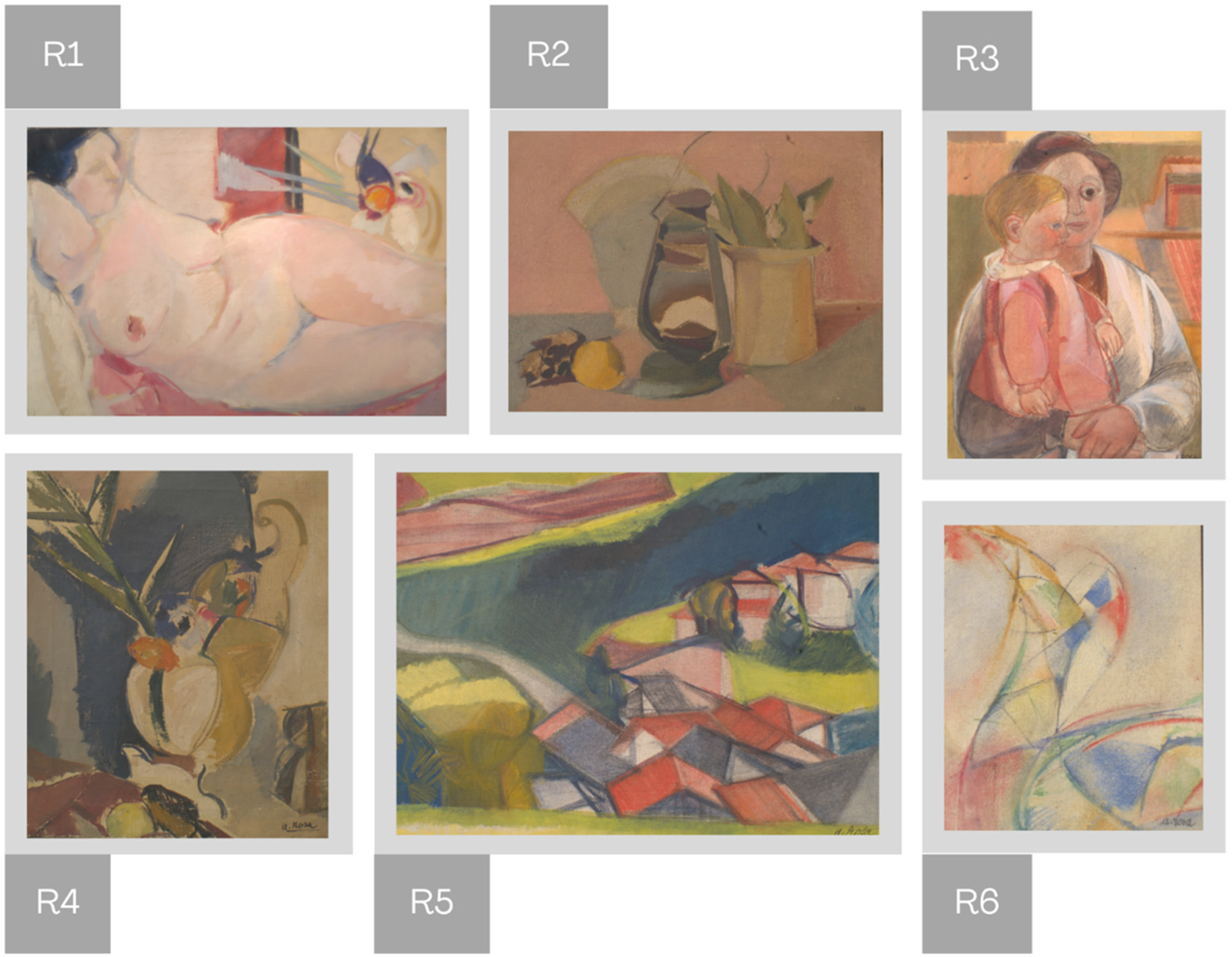
1.2. Andreina Rosa’s Paintings Included in this Study

Born in Venice, Andreina Rosa (1924–2019) was raised in an artistic context, with her father, Umberto Rosa, being a sculptor and a goldsmith. Consequently, she decided to delve into the study of art at the Instituto d’Arte dei Carmini and then at the Accademia di Belle Arti di Venezia. She took part in numerous editions of the Biennale (1950–1970) [14] and despite being more of note within the field of Applied Arts, her paintings reflect her meticulous technique.

Six paintings signed by the artist that currently belong to the International Gallery of Modern Art Ca’ Pesaro in Venice (Italy), which is affiliated with Fondazione Musei Civici (MUVE), were selected for the present study, namely: Nudo Coricato (1948–1949), Natura morta con lanterna (1950–1953), Giulia con Michele (1954), Natura Morta (1954–1955), Case sul lago (1954–1955) and Variazione sul Tema Maiastra: Il Fiore per la Principessa (1989). All six paintings have been studied as part of the didactic Laboratory course “Conservation Science for Modern and Contemporary Art” (A. Y. 2020/2021) taught by Prof. Francesca C. Izzo at the Ca’ Foscari University of Venice (Master’s Degree in Conservation Science and Technology for Cultural Heritage), using a multi-analytical approach, but the results have been treated individually for each of them. Consequently, this study merged the obtained data to investigate the artist’s painting materials and the evolution of the color palette through time. Moreover, the purpose of the data was to provide validation of the results obtained through the application of the functions included in the paletteR package [11] in R. The artworks were considered appropriate for the present research as Andreina Rosa used vibrant colors and did not apply any protective coatings, a practice which has been previously proven to strongly influence the color appearance [15]. Figure 1 shows the paintings and their corresponding codes.

1.3. The Aim of the Research

Since artists tended to paint with commercial materials, such as paint tubes [1], the painting process was easier as the preparation of pigments through grinding and their dispersion in a binding medium was no longer necessary. This meant that mixing colors to achieve different hues was an optimal solution as the various paints were already applied on a color palette, so they could be easily combined. It was quite common to use red and green to obtain brown, or yellow and blue to obtain green, but at the same time to employ pure color versions of the paints in various regions of the paintings. Therefore, nowadays, conservation scientists are faced with the problem of whether the paint layers that they analyze are made of a single chromophore pigment or combinations of two or even more that are found on the surface of the canvas. This leads to additional tasks in the analytical process as more samples are required and more spots within the artworks must be investigated. Therefore, this study aimed to examine whether K-means clustering applied using the paletteR package [11] in R could help in the preliminary identification of mixtures of pigments from the acquired images of Andreina Rosa’s paintings. Thus, colors were extracted from the images that have been previously corrected and simulations of mixtures were created. This could give preliminary answers prior to the use of any other scientific technique regarding the possibility of paint being a blend of two or more pigments that are present within the painting. Acknowledging the presence of a mixture might diminish the need to collect a sample both from the primary and the secondary/tertiary/composite colors, since the latter would also give the necessary information about the constituent primary colorants.

2. Materials and Methods

2.1. The Multi-Analytical Investigations for the Identification of Painting Materials

2.1.1. Fiber-Optics Reflectance Spectroscopy (FORS)

The instrument that was employed for carrying out the FORS analysis was an ASD FieldSpec 3 (ASD Inc., Alexandria, VA, USA), which is a portable, compact Fiber-Optics Reflectance Spectrometer, and can measure over a broad spectral range, namely from 350 to 2500 nm. The spectral resolution is differentiated in accordance with the wavelength, namely 3 nm (Full-Width-Half-Maximum) at 700 nm and 10 nm (Full-Width-Half-Maximum) at 1400 and 2100 nm. The benefits of the application of this technique mainly stemmed from the calculation of the first derivative from the registered spectra, which allowed the identification of some inorganic pigments and additives.

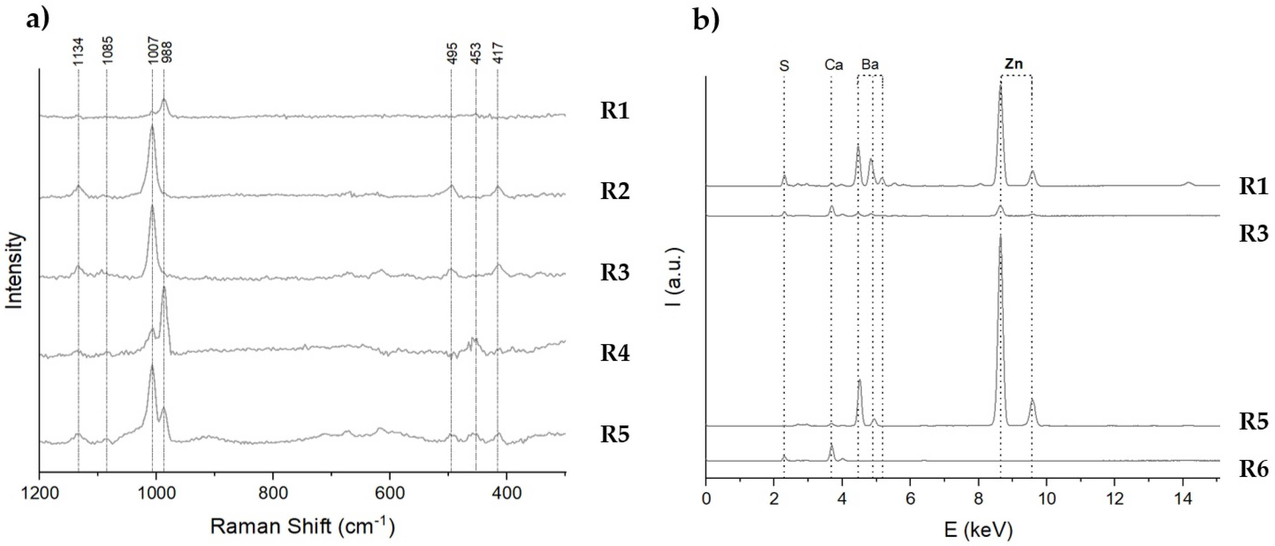
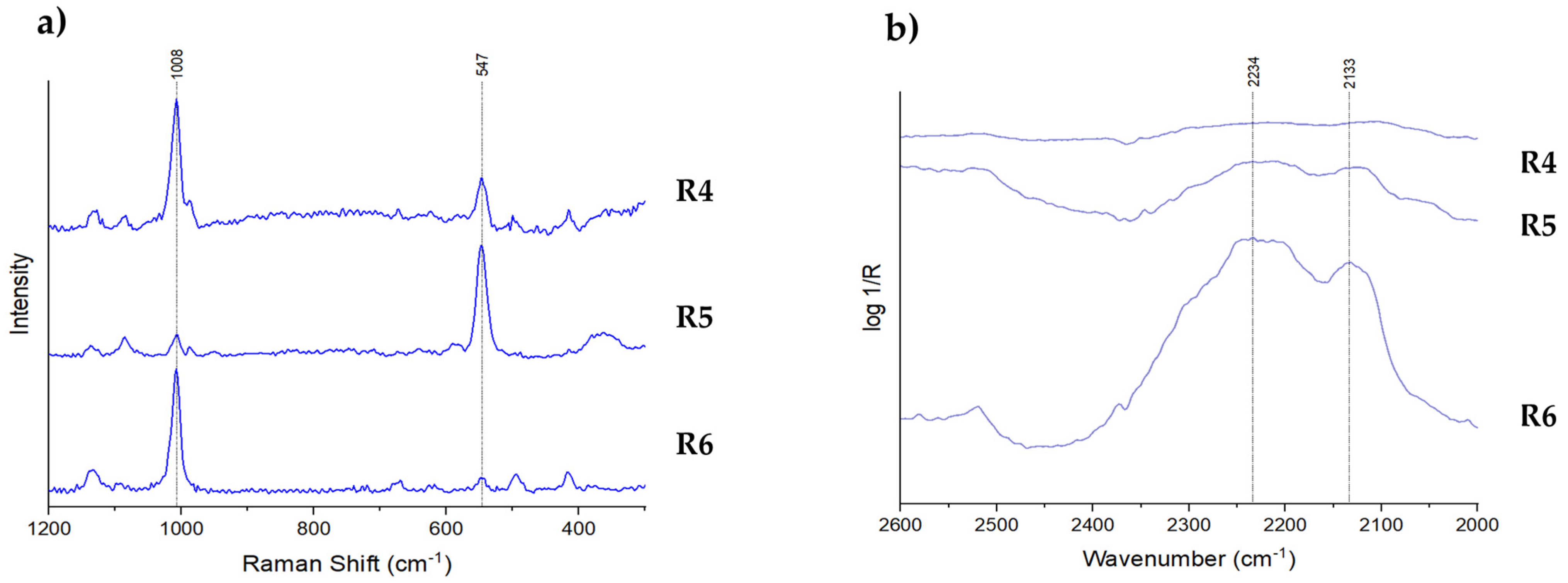
2.1.2. Raman Spectroscopy

Raman spectroscopy was performed using a BRAVO Handheld Raman Spectrometer (Bruker Optik GmbH, Ettlingen, Germany). The instrument is equipped with a dual-laser excitation, which can provide a simultaneous double excitation at 785 and 852 nm. Its spectral resolution is 10–12 cm⁻¹. Raman spectra were registered in the 3200–300 cm⁻¹ spectral range with a scanning time from 1 s to 300 s. It should be noted that the diameter of the tip of the instrument was 5 mm. This generally allowed the isolation of the analyzed colors, which led to the preliminary identification of some of the employed pigments. The only exception was the smallest painting, namely R6, that presented some brushstrokes which had a length of less than 5 mm, and thus the measurements and correct detection of the painting materials could not be made properly. The elaboration and the interpretation of data involved the use of three pieces of software: OPUS (version 8.2 provided by Bruker Optik GmbH), Spectragryph (version 1.2.16.1), and Origin Pro 2021 (version 9.8.0.200).

2.1.3. External Reflection FTIR Spectroscopy (ER-FTIR)

ER-FTIR analysis was employed mainly to strengthen the results obtained through Raman spectroscopy and obtain further confirmation of the presence of mixtures, when needed. This spectroscopic technique was applied on all artworks except for R6, as its surface was too small to allow adequate measurements. The spectra were recorded in the 7500–350 cm⁻¹ range using an ALPHA II Fourier Transform IR Spectrometer (Bruker Optik GmbH). The analysis points were investigated with 128 scans and a resolution of 4 cm⁻¹. The instrument was used at an aperture of 6 mm and the acquisition time was set to 3 min.

2.1.4. Energy Dispersive X-ray Fluorescence Spectrometry (XRF)

EDXRF was used for the preliminary identification of inorganic pigments and additives, except for R4, which was characterized by too high a degree of paint detachment for its safeguarding to be ensured throughout the analysis. The CRONO non-contact micro-XRF scanning spectrometer (provided by Bruker Optik GmbH) was employed as it ensured the stability of the artworks due to them being placed horizontally. It can detect all the elements ranging from sodium (Na, Z = 11) to uranium (U, Z = 92) both below 2 keV and above 25 keV. Moreover, it allows both punctual and areal analysis, rendering the creation of maps possible. The instrument was set to a voltage of 40kV, a current of 10 uA and a time frame of 90 s, the latter being high enough to prevent noisiness in the spectra. The 0.5 and 1-mm collimator apertures were used and the scanning area for generating the maps was approximately 30 mm × 30 mm.

2.2. The Computational Approach for the Identification of Mixtures

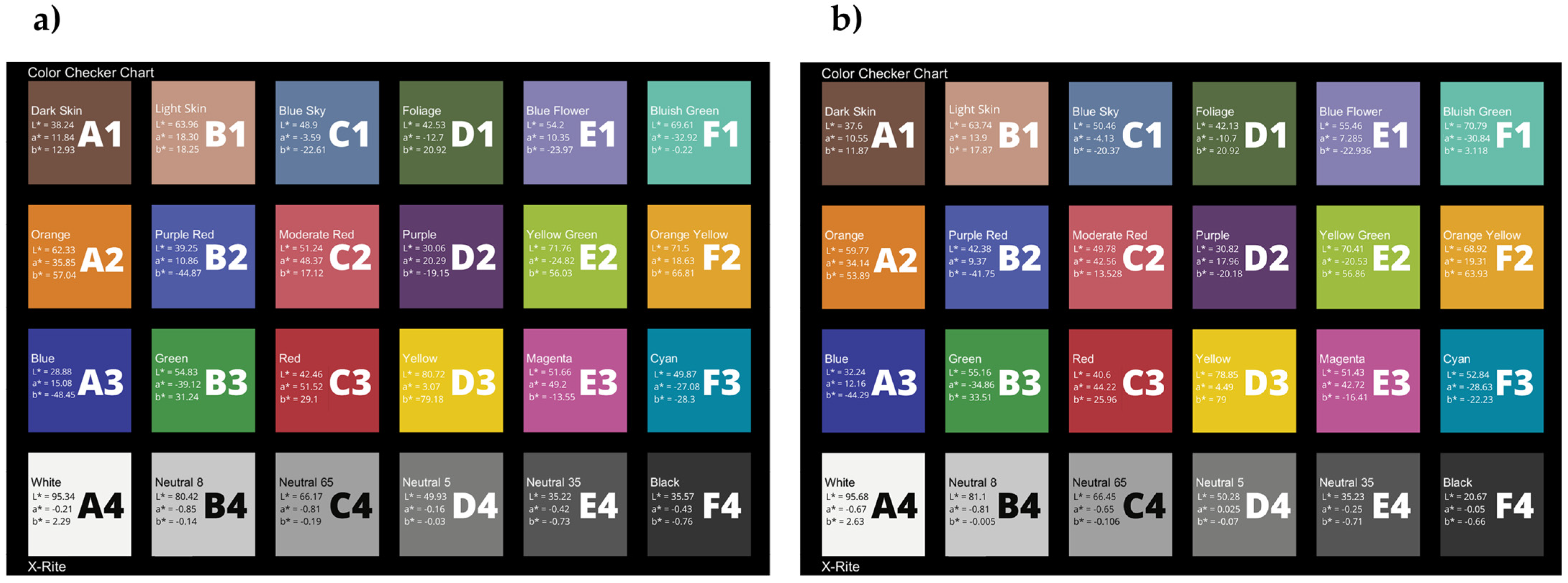
2.2.1. Camera, Lenses, and Color Target

The main problem that was faced when setting-up the equipment was the lack of a completely dark room in which light could be properly controlled. However, the images were shot at around noon on sunny days to obtain proper lighting that mimicked a probable lack of a dark room in the case of many museums and collections around the world. As a result, photos had to be subsequently transformed so as they all matched the conditions under the D65 standard illuminant. The photos were taken with a modified full-spectrum digital camera that was equipped with the UV/IR cut-off filter placed in front of the sensor. The camera that was used was Samsung NX3300 (which was modified by MADAtec Srl—Pessano Con Bornago, Italy) equipped with a CMOS sensor. The lens that was mounted on the camera was acquired from Olympus (Tokyo, Japan). The camera was fixed on a tripod and placed at a 50 cm distance from the paintings. The images were taken in the sRGB color space and saved in a RAW format. Their resolution was 3648 × 5472, and they had a 16-bit quantization level. The performance level of the images was, thus, kept between two and three stars, according to the FADGI (Federal Agencies Digitization Guidelines Initiative) guidelines, which were elaborated in the USA [16], as the digital camera allowed a maximum of 5472 pixels on the long dimension, which corresponds to the former level. The camera settings are included in

Table 1. Camera Setup.

Variable	Value
Flash	Off
ISO	400
Operation Mode	Manual
Exposure Time	1/125
Quality	RAW
f-stop	1.0
Color Space	sRGB

.

In order to further calibrate the images to obtain a more accurate reproduction, the ColorChecker^® Classic Mini Target (CC) created by X-Rite [17] (see Appendix A, Figure A1) was introduced in all images to act as a colorimetric reference. Since this color chart was manufactured to cover 24 of the most common colors in photographic and industrial applications [18] and the paintings of Andreina Rosa were characterized by a narrow color palette, this color chart was considered enough for the image analysis. However, when a wider range of colors is observed within the examined artworks, the Digital ColorChecker SG [19] color chart is recommended as it consists of 140 color patches. The CC that was used in this study was specifically bought for performing this image analysis. It should be noted that it has been kept almost entirely in its pouch to avoid any color degradation.

2.2.2. Spectro-Colorimetry

Spectro-colorimetry was performed for obtaining the chromatic L*a*b* coordinates of each of the color patches of the employed color target. These coordinates were useful for the subsequent correction of the images. In accordance with the CIE standard definition [20], the measurements were carried out using a Konica Minolta CM-26d Spectrophotometer in conjunction with SpectraMagic NX software with the following setups: illuminant D50, standard observer at 2° and illuminant D65, standard observer at 10°, both being acquired in SCI, as it is also summarized in

Table 2. Konica Minolta CM-26d Spectrophotometer Setup.

Variable	Value
Standard observer	2°/10°
Illuminant	D50/D65
Acquisition	SCI

.

D50/2° was used for computing the difference between the reference values provided by X-Rite for the ColorChecker® Classic Mini Target (post-November 2014–D50/2°) [21] and the values of the same color chart (manufactured in 2019) measured with the spectrophotometer in order to calculate the color difference between the two measurements and to check whether the color accuracy mean (CIEDE2000) was less than 2, which underlines the highest performance level (4 stars) according to the FADGI guidelines [16]. D65/10° was employed for the further calibration of the images, as they were taken in outdoor daylight conditions (D65) (see Appendix A, Figure A1). Four regions of each of the 24 patches were measured according to Figure 2; hence, a total of 96 regions were analyzed. For each region, three consecutive color measurements were made and then the average reading was calculated in order to avoid measurement errors [22]. The acquisition time for each measurement was 10 s.

2.2.3. Image Correction

The acquired images were directly implemented in the Imatest Master software (version 2021.2.6) [23], as the white balancing step is included within the color correction procedure. Despite the recommended use of a gold standard image that only contained the color chart, each photo was analyzed separately by manually selecting the ROI that included the CC as the light conditions suffered multiple changes throughout the taking of the images and a standard would have falsely reported the colors. The color correction matrix (CCM) was generated for the correction of the images in accordance with the reference values of the color checker (D65/10°) [24]. The type of CCM was chosen as 3 × 3, as the 4 × 3 option takes more time to process and it does not generally lead to better results. The color error metric that was selected for measuring the standard color error was ΔE₀₀ (CIEDE2000) [25] and the weight of the patches was set in accordance with the luminance value (L*). Linearization, which was carried out before the calculation of CCM implied a third-order polynomial fit to the common logarithm of the grayscale color patch levels [24]. The choice of this linearization was made as it did not require any prior knowledge regarding the encoding of the input image and it could be applied to a multitude of images, without affecting the accuracy of the results. The calculation was set to be made so as the XYZ matrix was found first from the input RGB values of the image and then converted to L*a*b* [26,27], the matrix being adjusted until ΔE₀₀ was minimized. Therefore, upon the completion of the optimization, the XYZ values were converted to the output RGB values.

2.2.4. The Application of K-Means Clustering Using the PaletteR Package

The paletteR package in R that uses K-means clustering for the extraction of colors from an image, which was created by Andrea Cirillo, follows five main steps, namely: the attribution of each pixel to a color cluster (a); the measurement of the centroid of each cluster (b); the change in data attribution according to the established centroid so that data points are as close to it as possible (c); the measurement of the Euclidean distance within clusters and its summing up in order to observe the performance of the obtained clusters (d); steps (b), (c) and (d) are repeated until the sum of distances is the lowest possible [12]. This process was applied to all six corrected images. However, the main issue with K-means is to determine the best K, i.e., the right number of color clusters to be extracted. This can be a significant drawback of its application on images of artworks because the quality of the results relies on the selection of K and the initial centroids [22,23]. The selection of the K value is crucial for ensuring an optimal clustering [28]. Indeed, different values for K may lead to different results. One of the available approaches is thus to run the algorithm multiple times by changing the K value until the best result is obtained. Since data here consisted of pixels that were rendering the colors of the images that represented the artworks, the determination of the number of K clusters, and of centroids, implicitly required multiple reiterations in accordance with the number of colors that were visually observed in the paintings.

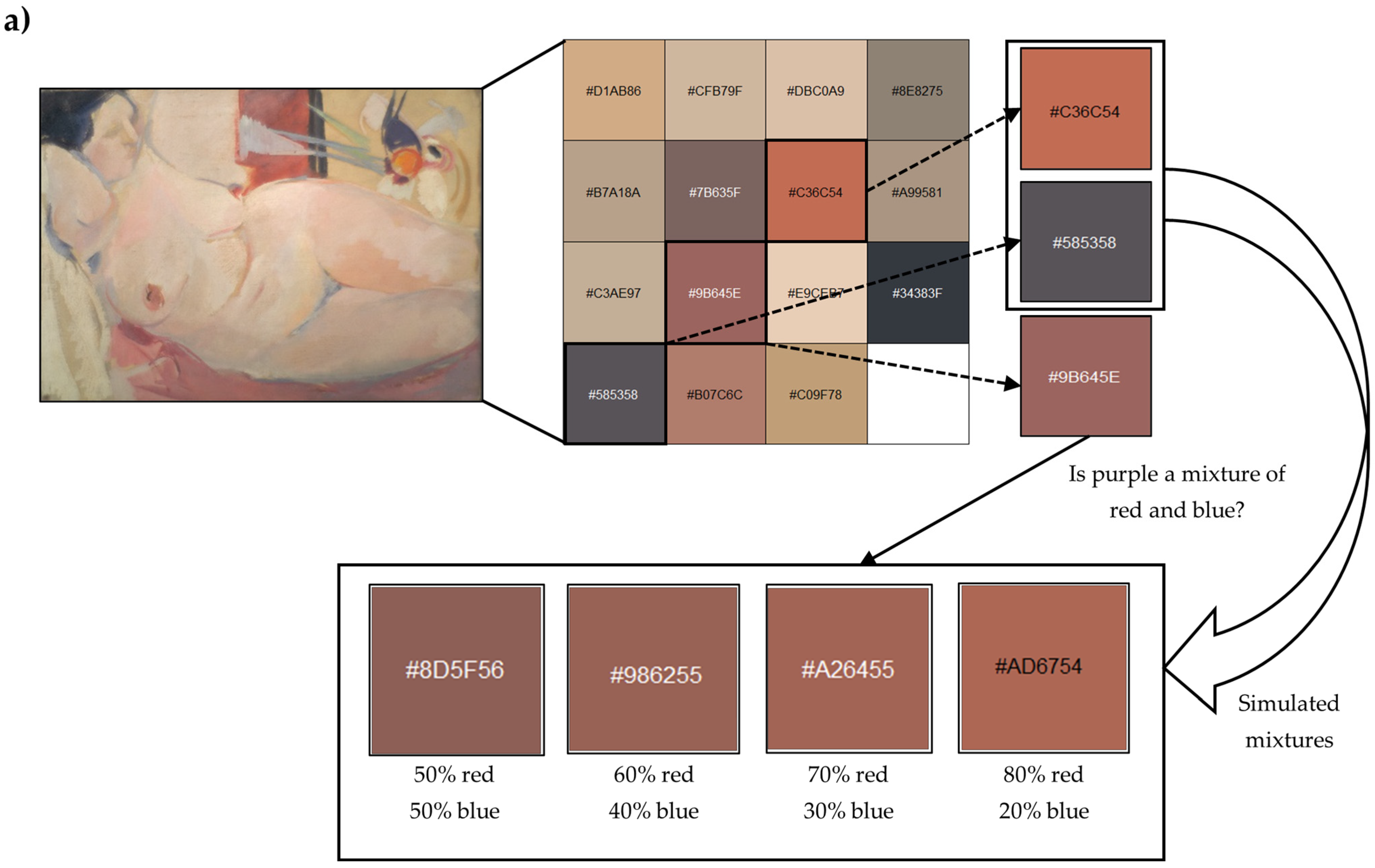
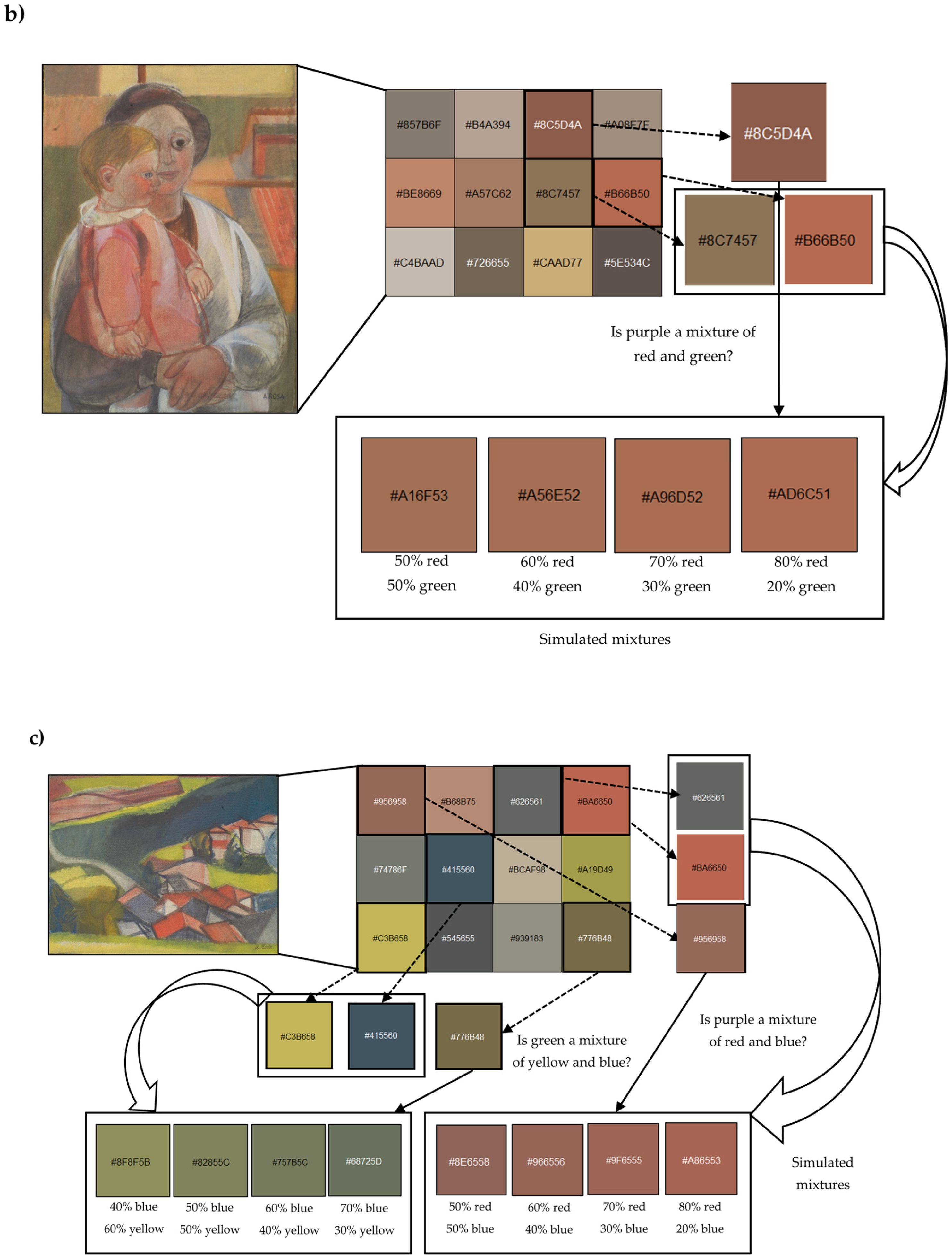
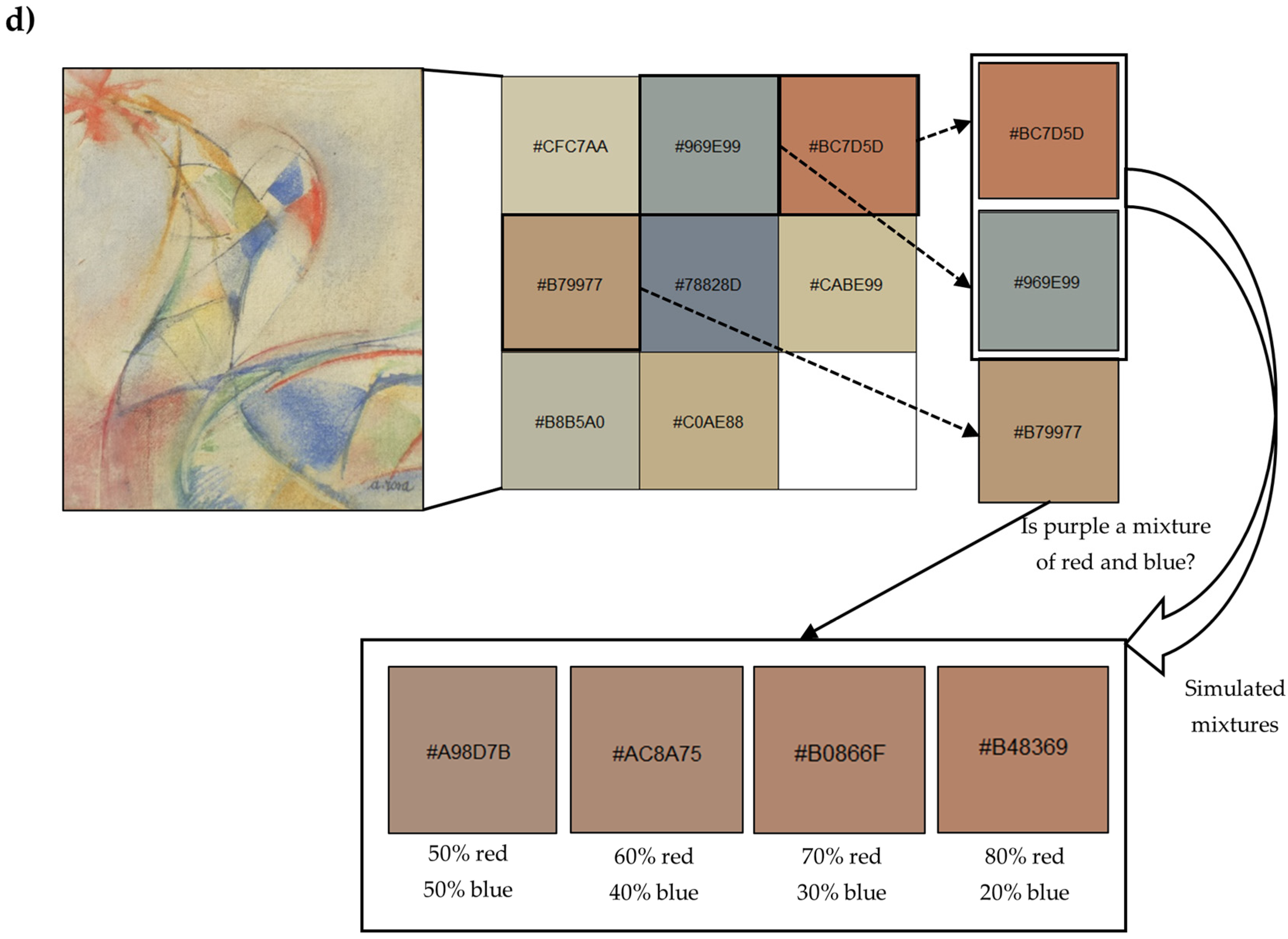
2.2.5. Simulation of Mixtures

The preliminary identification of mixtures of pigments was attempted using the colorspace package [29], which allowed the combination of two/three colors that resulted from the clustering analysis by employing the mixcolor function. Those colors were considered to represent pure pigments, since it was assumed that artists frequently combined paints deriving from various paint tubes to obtain colors such as green, orange, brown etc. or to achieve a brighter or a darker hue by adding white and black, respectively. This hypothesis was strengthened by the analytical campaign that emphasized this tendency of the artists to mix paints to obtain a new color.

2.2.6. The Measurement of the Color Difference

For comparing the RGB values extracted by R through K-means clustering with the colors corresponding to the simulated mixtures, the CompuPhase metric was employed, which measures the distance between two colors in a manner similar to the one in which a human being would perceive these distances. The equation (that measures the Similarity score) that describes this difference is:

$$Similarity score=\sqrt{\left(2+\frac{\overline{r}}{256}\right)\mathsf{\Delta }{R}^2+4\mathsf{\Delta }{G}^2+\left(2+\frac{255-\overline{r}}{256}\right)\mathsf{\Delta }{B}^2}$$

(1)

where $\overline{\mathrm{r}}$ is the mean of the red channel level between the two colors, and ΔR, ΔG and ΔB show the differences between the corresponding color channel values of the two colors. The lower this value, the more similar the colors are. Usually, a score of 100 or less is viewed as indicating a match [30]. This formula is also known as color approximation distance (CAD) as it weighs the RGB values in order to better match human perception and, thus, obtain a more adequate color approximation [31]. The similarity score was derived from several tests on 64 colors. The drawback is that it was not published in a formal article [32] and the experimental data are mainly unavailable to the users [33]. In spite of this, because it proved to give more accurate color differences than other formulas using the RGB coordinates, it was applied in this study in R through the colorscience package [34], which offers methods and data for color science, such as color conversion by observer, illuminant and gamma.

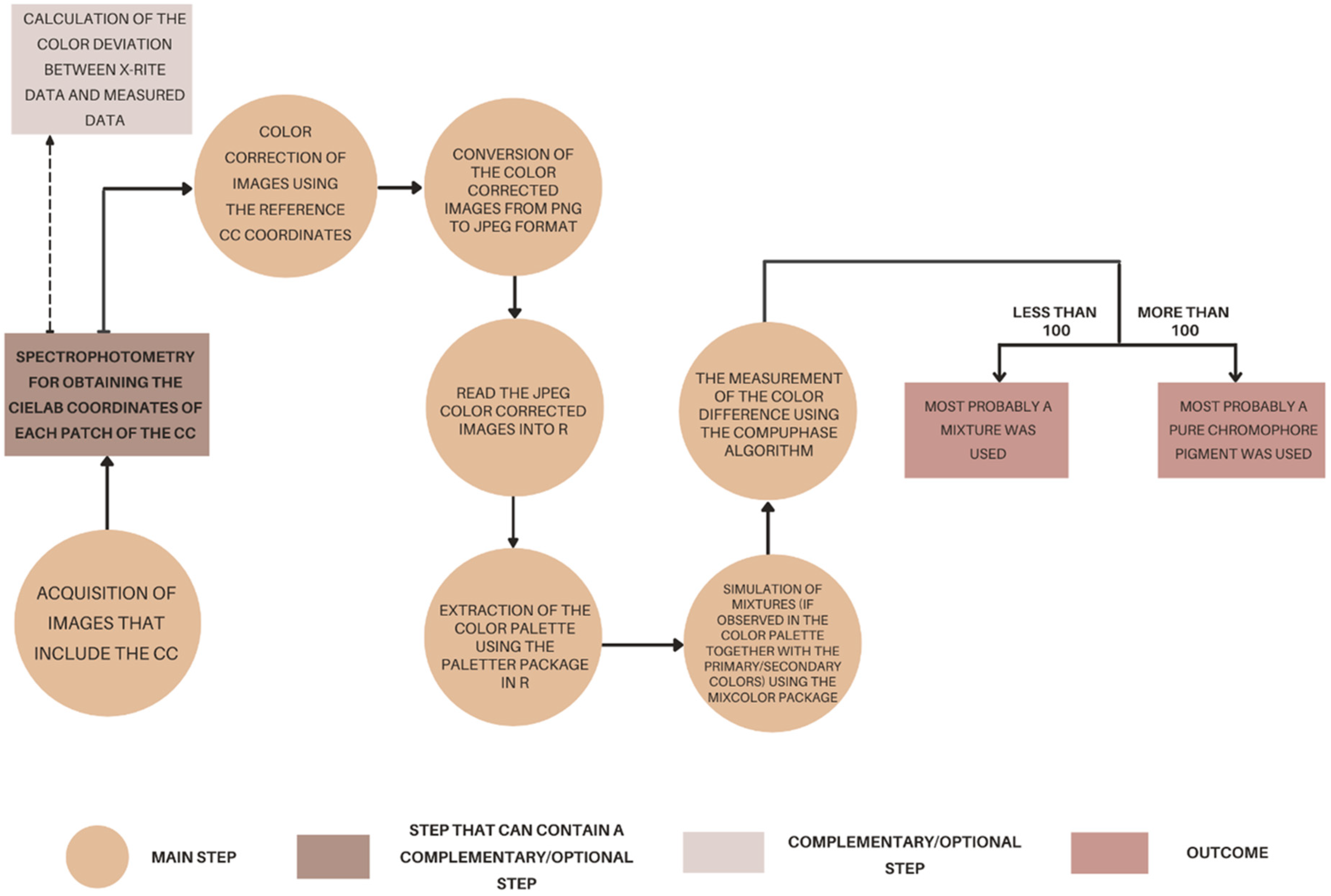
2.2.7. Summarized Workflow

Figure 3 summarizes the steps that were undertaken in the proposed method that go from the acquisition of the images to their correction using the color target (CC) that had been calibrated and finally to the extraction of the colors using K-means clustering, the simulation of the mixtures and the measurement of the color differences between the originally extracted secondary/tertiary/composite colors and the simulated ones. The packages that were used for image analysis in R (version 4.0.2) besides paletteR [11] (version 0.0.0.9000) were colorscience [34] (version 1.0.8), colorspace [29] (version 2.0-0), jpeg [35] (version 0.1-8.1.), and magick [36] (version 2.5.2.).

3. Results and Discussion

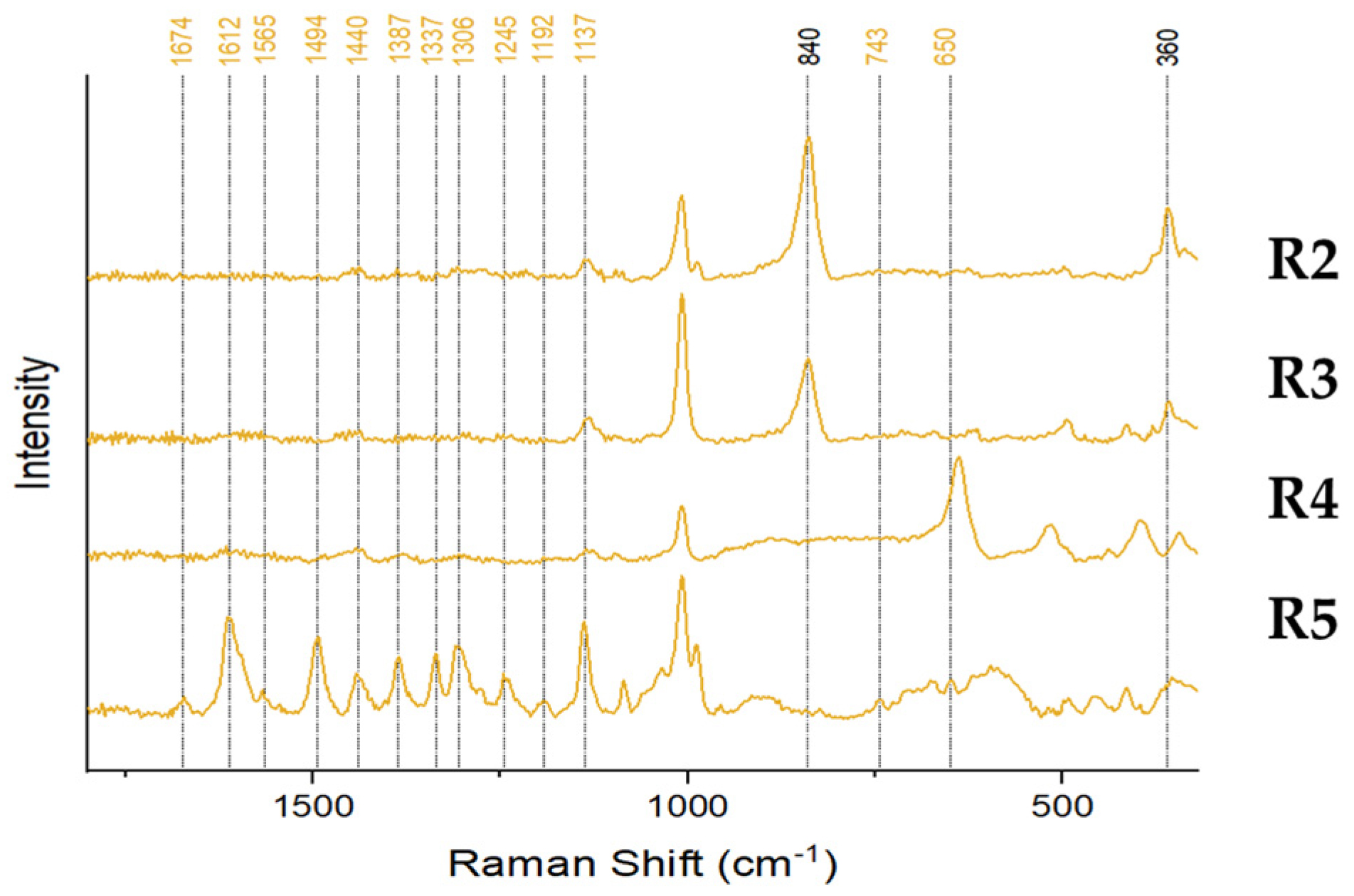
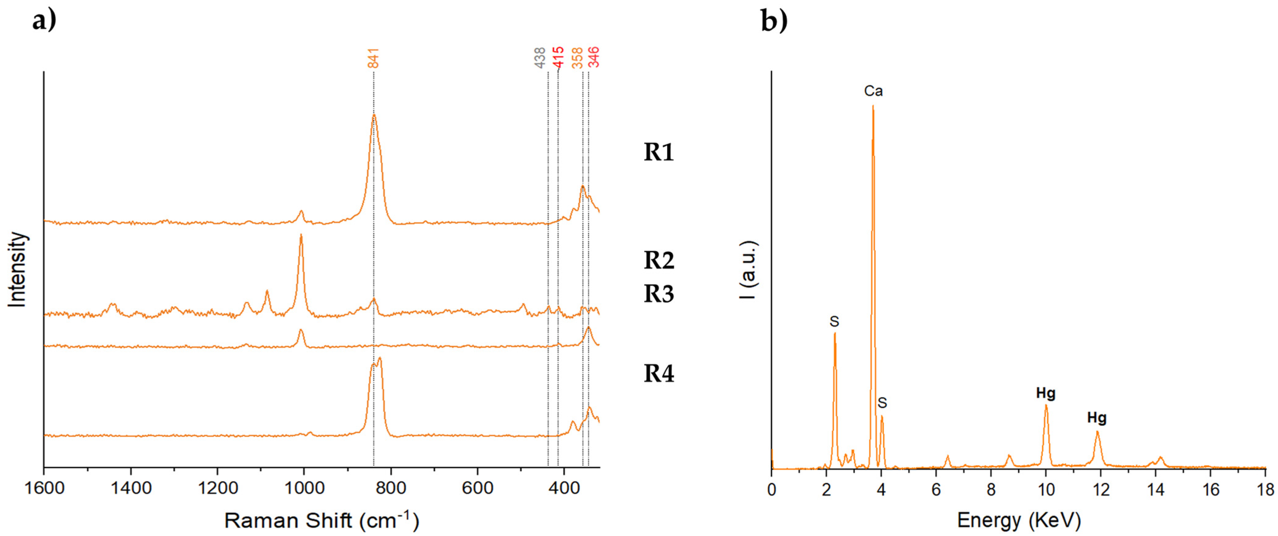
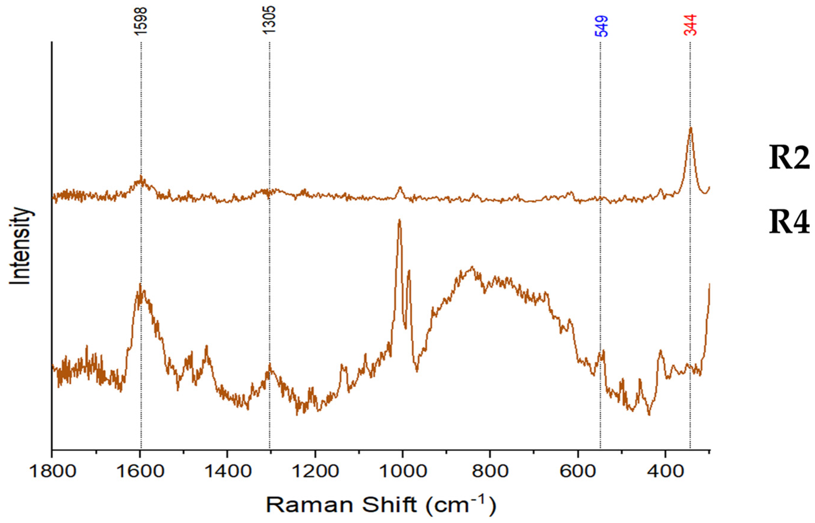
3.1. The Pigments used by Andreina Rosa

3.1.1. White Pigments

White paint was predominant in all six paintings, and it mainly consisted of components that were generally found in the ground layer, namely gypsum, barium white/lithopone and calcite. This might emphasize the predilection of the artist for a preparatory layer that acted both as a primer and a white paint. Consequently, all the other paint layers were applied on top of it, probably to trigger a watercolor effect. The recorded Raman spectra (see Appendix B, Figure A2a) underline the use of gypsum, which could be easily observed at 1134, 1007, 495 and 417 cm⁻¹ [37]. The spectra of the white paint of R2, R4 and R5 might indicate traces of calcite at 1085 cm⁻¹. Nonetheless, other analytical techniques such as ATR-FTIR should be applied in order to fully confirm its existence within the preparatory layers. No distinction could be made between barium white and lithopone, as they are characterized by similar bands. They could be identified at 988 and 453 cm⁻¹ in all artworks except for R2 and R3. Nevertheless, it is highly likely that Andreina Rosa generally used lithopone as a white pigment since the specific Raman signals of other commonly employed pigments in modern and contemporary art, such as zinc white, lead white and titanium white, could not be identified. Moreover, the results were confirmed through XRF (see Appendix B, Figure A2b) [38], which emphasized the presence of the following elements in R1 and R5: sulfur (S) due to the peak at 2.3033 keV (Kα₂) and barium (Ba) due to the peaks at 4.4681 and 4.8311 keV (Lα₁ and Lβ₁). However, zinc (Zn) was also detected in both paintings at 8.6423 and 9.6016 keV (Kα₁ and Kβ₁), which provides a further confirmation of the use of lithopone (ZnS + BaSO₄). The presence of calcium (Ca) at ca. 3.69 keV (Kα₁ and Kα₂) should also be noted since it might additionally highlight the use of gypsum (CaSO₄ · 2H₂O) as a main component of the preparatory layers. Thus, the sulfur detected through XRF might suggest the existence of both lithopone and gypsum.

3.1.2. Blue, Green, and Purple Pigments

R4, R5 and R6 presented an abundance of blue paint that was identified as being mainly composed of ultramarine blue, which was underlined by the Raman peak at 547 cm⁻¹ that is specific for the symmetric stretching vibration (ν₁) of the S₃⁻ ion present in lazurite [39] (see Appendix B, Figure A3a). The nature of the ultramarine blue pigment, namely natural or synthetic, was mainly examined through reflection infrared spectroscopy (ER-FTIR). According to [40,41,42,43], the pigment seemed to be synthetic because of the lack of the characteristic sharp band at 2340 cm⁻¹, which might be attributed to the CO₂ molecules entrapped in the sodalite cages of the natural mineral pigment (lazurite) from Afghanistan, Iran and Siberia (see Appendix B, Figure A3b). FORS, which is also used to determine the nature of ultramarine blue, could not additionally confirm the synthetic nature of the pigment since it was highly probable that it had been mixed with lithopone, which led to a bathochromic shift in the specific peak to the artificial version at ca. 450 nm to longer wavelengths [44]. However, invasive analysis is required to fully discriminate the two versions of ultramarine blue, such as optical microscopy (OM) or high-magnification Scanning Electron Microscopy (SEM) [39]. Nevertheless, it is very likely that Andreina Rosa used commercial paints, hence ultramarine blue being artificial.

Moreover, ER-FTIR allowed the identification of the reststrahlen band at around 1010 cm⁻¹, which was attributed to the asymmetric stretching of Si,Al-O within the constituent tetrahedra [41] (see Appendix B, Figure A4). This band was detected in the case of the purple pigment of R1 and the green pigment in R5, underlining the high probability of a mixture of blue and red and of blue and yellow, respectively. However, the presence of cinnabar red and Hansa yellow could not be confirmed through this technique.

Purple paint Raman spectra were characterized by noise most probably because of the presence of carbon-black (D and G bands were identified at 1310 and 1603 cm⁻¹) that absorbed or radiated light [45] (see Appendix B, Figure A5a). This pigment was likely added by the artist herself to darken the color. The presence of ultramarine blue could be detected at 548 cm⁻¹, but the red counterpart of the color could not be observed. Hematite could be clearly observed in R2 due to the presence of the two peaks at 613 and 414 cm⁻¹ that are assigned to the α-Fe₂O₃ vibrations [46]. These two peaks might have been present in R1 and R5 as well, but they are not well defined. XRF results indicated the existence of one of the most important emission lines of iron (Fe), namely at 6.3867 keV (Kα₁) in the case of R5, that might confirm the presence of hematite. However, there was also an emission line that might suggest the presence of mercury (Hg) at 14.1517 keV (L_iiab), which could underline the presence of vermilion (see Appendix B, Figure A5b), thus suggesting a high probability for a mixture of this red pigment and ultramarine blue for rendering the purple color. This result seems to highlight the use of a combination of pigments that were most probably also applied individually for depicting the purer paint layer, such as the blue or red paint layer, for rendering the purple color in the case of R1, R2 and R5.

3.1.3. Red Pigments

XRF indicated the predominance, in red areas, of cinnabar red in the case of R3 and R5 due to the presence of the characteristic peaks for mercury (Hg) at 9.9905 keV (Lα₁) and 11.8227 keV (Lβ₁) (see Appendix B, Figure A6a). This result was confirmed by Raman, as can be seen in Appendix B, Figure A6b, the specific band at 344 cm⁻¹ being present in both paintings. In R1 and R4, studio red Hansa pigment (C₁₇H₁₃N₃O₃) was found, emphasized by the wavenumbers at 1618, 1556, 1497, 1396, 1445, 1329, 1252, 1220, 1184 and 1129 cm⁻¹ that were consistent with those reported by Burgio et al. [37]. Studio red Hansa pigment is also known as Hansa Scarlet RNC or Pigment Red 3 (PR3), and it is a β-naphthol-based synthetic organic pigment [47] that was made available in 1905 and is still employed in domestic and industrial paints and in colors for printing [48]. However, no other case study was found in the literature that underlined its use as an artist’s pigment. Raman spectroscopy did not provide a clue for the identification of the red pigment in the case of R6, thus FORS was employed for evaluating the potentiality of the first derivative to provide information. Consequently, the spectrum (shown in Appendix B, Figure A7a) presented a positive slope at around 550 and 600 nm, a slope characterized by sharpness, which is specific to hematite (Fe₂O₃). Moreover, the first derivative (shown in Appendix B, Figure A7b) indicated a maximum peak at 580 nm, which is within the typical range (575–580 nm) for red ochre that consists of hematite (Fe₂O₃) [49]. Furthermore, the XRF spectrum suggested the presence of iron (Fe) at 6.4126 keV (Kα₁) that might emphasize the usage of hematite. It should be noted that this specific signal was observed only in the case of R6, strengthening the presence of red oxide as it may not seem to be characteristic of the ground layer.

3.1.4. Yellow and Orange Pigments

The artist preferred the use of both inorganic and organic yellow paint, the former being visible in the case of R2 as the two characteristic Raman wavenumbers for chrome yellow (PbCrO₄) could be found at 840 and 360 cm⁻¹ [50]. Hansa yellow, which is a synthetic organic pigment, could be identified solely in R5, most probably in the form of PY3 (C₁₆H₁₂C_l2N₄O₄). This could be explained by the presence of two bands that are not specific to PY1 (C₁₇H₁₆N₄O₄), the other common form of Hansa yellow, namely the 744 cm⁻¹ band that is attributed to the C-H bending and the 650 cm⁻¹ band that is assigned to the C-Cl stretching [51]. The other specific bands for Hansa yellow are depicted in Appendix B, Figure A8. Despite the low intensity of the peaks in R3 and R4, the wavenumbers seem to correspond to those observed in R5, thus they might also emphasize the use of the Hansa yellow pigment. It should be noted that the signals for anatase in the case of R3 might cover the intensity of the other peaks.

The Raman spectra for the orange paint (see Appendix B, Figure A9a) of R1, R2 and R4 implied the presence of chrome yellow (PbCrO₄), as the two peaks corresponding to it were well defined (841 and 358 cm⁻¹). The wavenumber at 346 cm⁻¹ suggests the existence of cinnabar red (HgS), which seems to be the sole chromophore pigment in the orange paint spectrum of R3. Moreover, in the case of the latter the pigment is also confirmed by the XRF signals at 9.9905 and 11.8442 keV which correspond to Hg (Lα₁ and Lβ₂) (see Appendix B, Figure A9b). The peak at 438 cm⁻¹ that could be observed in the case of R2 might indicate the additional presence of zinc white (ZnO). The band at 415 cm⁻¹, which was visible only in the case of R2 might be attributed both to gypsum (CaSO₄ · 2H₂O) and hematite (Fe₂O₃). However, the other characteristic peak for the latter at around 610 cm⁻¹ could not be identified.

3.1.5. Brown Pigments

Brown paint was found in only two paintings, namely R2 and R4, as both exhibited the two characteristic Raman bands of a carbon-based black pigment (see Appendix B, Figure A10). The D-band could be observed at 1598 cm⁻¹, whereas the G-band at 1305 cm⁻¹ [37]. The crystalline form of graphite is described by a single narrow band near 1350 cm⁻¹ (G stands for ‘graphite’), whereas the disordered form of graphite additionally includes a band at around 1598 cm⁻¹ (D stands for ‘disorder’) [52]. It should be noted that in R2, the peaks are less intense than in R4, as the former also comprises cinnabar red, visible at 344 cm⁻¹. However, it appears that brown has been obtained through the mixture of red and green only in the case of R4, as no characteristic band for green could be found, nor implicitly for yellow and blue in R2. The peak at 549 cm⁻¹ might correspond to ultramarine blue, but it should be noted that since the spectrum was noisy, the presence of the yellow pigment could not be confirmed. Moreover, brown paint was also observed in R3, but the registered spectra had a noisy nature, which limited the detection of the 344 cm⁻¹ wavenumber that corresponded to cinnabar red and the D and G bands of carbon-black pigments.

3.1.6. The Color Palette of Andreina Rosa

The artist seems to have preferred oil paints according to Piccolo et al. [53], which were most likely directly procured in the form of paint tubes, judging by her quick brushstrokes, especially in the case of R5, which is a landscape, and it is highly probable that it was painted in plein-air. Moreover, her color palette is narrow, generally comprising of primary colors and neutral colors, as she opted for mixing to obtain secondary/tertiary/composite colors and modulate their brightness or darkness. The pigments that have been identified in the six analyzed paintings are shown in

Table 3. The color palette of Andreina Rosa.

Color	Pigments
White	Lithopone
Black	Carbon-black
Red	Cinnabar red
	Studio Hansa red
	Hematite
Blue	Ultramarine blue
Yellow	Chrome yellow
	Hansa yellow (PY3)
Purple	Hematite or cinnabar red, ultramarine blue and carbon-black
Green	Ultramarine blue and Hansa yellow
Orange	Chrome yellow and cinnabar red
Brown	Cinnabar red, ultramarine blue, and carbon-black

.

3.2. The Preliminary Identification of Mixtures

3.2.1. The Color Correction of Images

It should be noted that prior to the insertion of the images in the Imatest Master software (version 2021.2.6) [7], the color target was studied to understand the differences between data provided by the X-Rite company and customized data obtained through spectro-colorimetric measurements (see Appendix A, Figure A1). This approach had as its main outcome the identification of the magnitude of the color deviations.

Table 4. CIEDE2000 color difference between the CIELAB coordinates (D50 illuminant, 2° standard observer) provided by the X-Rite ColorChecker Mini chart supplier and the custom data of the same chart (D50 illuminant, 2° standard observer). The differences are marked using colors, dark green representing a CIEDE2000 < 1, light green between 1 and 2, orange between 2 and 3, and red more than 3.

	A	B	C	D	E	F
1	2.057	1.154	0.464	1.329	1.252	0.729
2	0.395	0.263	0.733	1.247	0.909	0.346
3	0.607	0.586	0.214	0.823	1.215	1.23
4	1.275	0.921	0.598	0.841	0.423	11.33

highlights the color deviations for each of the 24 colors patches, the only value higher than 3 being registered for the black color patch (F4), which could be explained by the large variations in the L* coordinate corresponding to lightness [22]. In other words, the L*a*b* coordinates of this patch according to X-Rite were (20.64, 0.07, −0.46), whereas in this study they were found to be (35.57, −0.43, −0.76) emphasizing the substantial difference in the L* coordinate. Despite this, the average CIEDE2000 was calculated to be 1.28 when the black patch was included and 0.85 when it was excluded. As Kirchner et al. [22] suggested, the values reported by X-Rite for the black patch are not as high as they should be, but even if the color target were calibrated by the photographer, the L* coordinate would still be too high to be representative. As a result, this could lead to dark colors being shown as brighter than they are. The reference data that were inserted in Imatest Master corresponded to the D65 illuminant, 10° standard observer.

The procedure implemented in Imatest Master was straightforward and it easily allowed the generation of new images that respected the CIELAB values measured for the reference CC. ΔE₂₀₀₀, the color difference that was taken into consideration, proved to be between 6.49 and 12.72 prior to the processing of the images in the afore-mentioned software, thus being clearly perceptible. However, after the correction using the reference CC, ΔE2000 substantially decreased. The average color difference for all the analyzed paintings was calculated to be 3.68, which is within the acceptable range for commercial reproduction, namely between 3 and 6 [54]. This highlights the fact that, generally, the difference between the colors of the reference and the corrected color chart present in the images cannot be perceived by human vision, except for the situation in which two colors overlap. It is noteworthy that ΔE₂₀₀₀ was the highest in the case of R4, which could be explained by the predominance of darker paints. Therefore, the lack of proper L*a*b* coordinates for the black patch (F4) significantly increased the color difference.

The lowest ΔE₂₀₀₀ of all analyzed images was noticed in the photo of R5, namely a value of 3.19 (shown in

Table 5. The color difference (ΔE₂₀₀₀) in the input and output images corresponding to the analyzed artworks. The difference was measured between the reference CC and the colors present in the images. The green cell underlines the lowest registered color difference of all photos and the red cell vice versa.

Painting Index	ΔE2000 (Input-Reference)	ΔE2000 (Corrected-Reference)
R1	6.49	3.26
R2	11.09	3.39
R3	11.41	3.68
R4	12.72	4.48
R5	9.74	3.19
R6	10.9	4.09

and visually noticeable in Figure 4). The highest performance level according to the FADGI guidelines [16] was three stars and was obtained in four artworks of Andreina Rosa (R1, R2, R3 and R5). To the rest of the photos, a performance of two stars was assigned.

3.2.2. The Extraction of the Color Palettes Using the PaletteR Package in R

Since paintings were not protected by varnish layers, the outcome of the clustering analysis on the corrected images featured a satisfactory extraction of colors. The method proved to be efficient in the case of R1, R3, R5 and R6, as they were characterized by vibrant colors that covered a larger surface area of the canvas and, thus, could be identified. The extraction of the color palette from R5, the most optimally corrected image, gave a particularly satisfactory outcome (Figure 4) as all primary colors, namely red, blue, and yellow, could be individually extracted. However, it should be mentioned that red had not been uniformly applied on the preparatory layer, its paint layer being thin. Moreover, yellow veered towards green, which according to Raman spectroscopy, mainly consisted of Hansa yellow, which has a yellow–green color [55]. Consequently, mixtures could be simulated, namely purple and green, using the individual primary colors, red and blue, and yellow and blue, respectively. Despite this, the identification of the whole color palette was burdened in the case of R2 and R4 by the presence of a multitude of overlapping brushstrokes. Additionally, according to the analytical techniques, these two paintings consisted of paints that were characterized by traces of carbon-black pigments that rendered the colors darker. Thus, the extraction was not reliable, with typically only the background being identified, even when trials were performed using a higher number of clusters.

3.2.3. The Simulation of Mixtures and Measurement of Color Differences

Mixtures could be simulated in the case of four paintings, namely R1, R3, R5 and R6, which are shown in Figure 5 with their corresponding color differences in

Table 6. The CompuPhase color difference between the simulated mixtures and the previously extracted secondary/composite colors.

Painting Index	Percentage of Colors	CompuPhase Color Difference (K-Means)
R1	50% red + 50% blue	27.82
	60% red + 40% blue	12.95
	70% red + 30% blue	18.41
	80% red + 20% blue	36.28
R3	50% red + 50% green	26.45
	60% red + 40% green	31.08
	70% red + 30% green	41.78
	80% red + 20% green	55.25
R5	50% red + 50% blue	14.25
	60% red + 40% blue	7.69
	70% red + 30% blue	20.46
	80% red + 20% blue	36.02
	40% blue + 60% yellow	87.8
	50% blue + 50% yellow	63.07
	60% blue + 40% yellow	45.14
	70% blue + 30% yellow	42.88
R6	50% red + 50% blue	37.69
	60% red + 40% blue	37.25
	70% red + 30% blue	40.65
	80% red + 20% blue	47.03

. The only mixture identified through clustering in R1 was purple (Figure 5a), despite green also being present, but in a small amount according to the visual observations that was not considered significant by the algorithm. All similarity scores are even smaller than 40, which seems to strongly confirm the presence of a mixture, as was also pointed out in the first part of this study. Accordingly, a mixture of 60% blue and 40% red gave the best result, with a difference of only 12.95. However, it should be kept in mind that blue might not have been entirely pure as it might reflect the co-presence of black and white.

Brown was extracted only from R3 (Figure 5b) together with its constituent colors, namely red and green. However, green, a secondary color, could not be simulated as blue was not present as an individual color within the color palette obtained through clustering. The existence of the mixture was suggested especially by the 50% red and 50% green blend. Nevertheless, the only image that allowed the extraction of two secondary colors together with their corresponding primary components was R5, as shown in Figure 5c. Since purple was noticed mainly in the regions where red and blue were overlapping and the ground layer was visible, which might have enhanced the brightness of the color, the lighter blue was selected for the creation of the mixture. Conversely, in the generation of the green color, the darker blue was chosen, as the observed green hue on the surface of the canvas was vibrant and it seemed to lack white paint. The best color matches were simulated using 60% red and 40% blue for purple and 70% blue and 30% yellow for green.

In R6, all the extracted colors were brighter, which was probably due to fact that the painting was a watercolor and colors were not uniformly dispersed on the surface of the canvas. However, purple could also be simulated using the extracted red and blue colors. The chosen blue shade was light blue as it included the presence of white, matching the observed purple more, which seemed to include white as well (Figure 5d). The generated blends were quite satisfactory, as they presented color differences that were slightly less than 50, which might, thus, suggest the existence of a mixture of red and blue, composed of around 60% red and 40% blue.

Therefore, the clustering analysis applied to the images of Andreina Rosa’s paintings led to the identification of mixtures of pigments even if colors had been altered by the presence of white and black. However, there is a main limitation to this computational technique, namely the fact that the color of pigments depends on the chromatophores that are present in their structure. For example, the color of ultramarine blue is highly influenced by the S₃⁻/S₂⁻ ratio [56] since S₃⁻ absorbs within the yellow-orange region at ca. 590–610 nm, offering a blue color, whereas S₂⁻ provides a yellow hue, absorbing light at ca. 380 nm. Thus, if the concentration of these two ions varied, it would lead to a greener or a bluer color of the pigment. Ultramarine blue pigment that was mixed with red to obtain purple or with yellow to produce green might have been different. Therefore, the simulation of mixtures might not completely reflect this aspect, and this should be further studied.

4. Conclusions

In the framework of the analyzed modern and contemporary paintings of Andreina Rosa, the use of the paletteR package [11] for the extraction of colors and the subsequent simulation of mixtures proved to be useful only when the artworks satisfied the following conditions:

• They were unvarnished;
• They were not affected by substantial degradation that might have caused colors to fade or might have reduced the visibility of the original hues;
• The majority of paint layers was light and vibrant as the predominance of dark colors would imply a poor color correction of the image;
• The primary colors that could compose the visible mixtures are present on the surface of the canvas.

However, even if the artworks respect all the conditions, color correction is mandatory prior to the employment of K-means clustering to ensure color precision. Imatest Master software can easily provide the necessary support for the fulfillment of this task as it generates the CCM using the reference CC data. It has been observed that this pixel-based color segmentation methods employed using the paletteR package [11] can be effective. Moreover, K-means clustering gives particularly satisfactory results if the painting presents well-defined and separated colors.

Furthermore, mixtures could be simulated knowing whether they were indeed present in the paintings or not, according to the results provided by the analytical techniques. However, the proposed technique has some drawbacks that should be solved with further research. Firstly, the analysis of mock-ups is suggested to completely validate the method and confront the created mixtures from known pigments to the digitally simulated ones using the individual colors from the acquired images. Secondly, a comparison should be made between the original hue of the pigments (theoretical) and the real detected hue of the pigments as the chromatophore groups might clearly influence the observed colors. Thirdly, more modern and contemporary paintings should be examined using this approach since Andreina Rosa generally employed mixtures and, thus, the color difference was never observed to be beyond 100 in order to further verify the method in the case of the lack of mixtures as well.

Regarding further developments of the proposed technique, the efficiency of other clustering techniques such as e.g. Fuzzy C-means clustering [57] and dominant sets [58] could be tested especially in the case of modern paintings in which there are numerous overlapping clusters. Another expansion of the method would involve the conversion of colors from the sRGB color space to CIELAB, using the CCM matrices generated during the color correction procedure. This could lead to the establishment of a database in which the mixtures of artist paints could be provided together with their L*a*b* coordinates according to the binding medium in which they were dispersed. In addition, Bruce MacEvoy [59] has already created a chart of pigments that were averaged over various paint brands, but they were all watercolors and they were not mixed; thus, this could be developed to a greater extent to incorporate paints that were created using various binding media and the L*a*b* coordinates of their corresponding mixtures.

References

1. Izzo, F.C.; van den Berg, K.J.; van Keulen, H.; Ferriani, B.; Zendri, E. Modern Oil Paints–Formulations, Organic Additives and Degradation: Some Case Studies. In Issues in Contemporary Oil Paint; van den Berg, K.J., Burnstock, A., de Keijzer, M., Krueger, J., Learner, T., de Tagle, A., Heydenreich, G., Eds.; Springer International Publishing: Cham, Switzerland, 2014; pp. 75–104. [Google Scholar]
2. Hong, G.; Luo, M.R.; Rhodes, P.A. A Study of Digital Camera Colorimetric Characterization Based on Polynomial Modeling. Color Res. Appl. 2001, 26, 76–84. [Google Scholar] [CrossRef]
3. Bianco, S.; Schettini, R.; Vanneschi, L. Empirical Modeling for Colorimetric Characterization of Digital Cameras. In Proceedings of the 2009 16th IEEE International Conference on Image Processing (ICIP), Cairo, Egypt, 7–10 November 2009; pp. 3469–3472. [Google Scholar]
4. Trombini, M.; Ferraro, F.; Manfredi, E.; Petrillo, G.; Dellepiane, S. Camera Color Correction for Cultural Heritage Preservation Based on Clustered Data. J. Imaging 2021, 7, 115. [Google Scholar] [CrossRef]
5. Molada-Tebar, A.; Lerma, J.L.; Marqués-Mateu, Á. Camera Characterization for Improving Color Archaeological Documentation. Color Res. Appl. 2018, 43, 47–57. [Google Scholar] [CrossRef]
6. Gaiani, M.; Apollonio, F.I.; Ballabeni, A.; Remondino, F. Securing Color Fidelity in 3D Architectural Heritage Scenarios. Sensors 2017, 17, 2437. [Google Scholar] [CrossRef] [PubMed] [Green Version]
7. Imatest Master. Available online: https://www.imatest.com/products/imatest-master/ (accessed on 14 April 2022).
8. BabelColor–Color Measurement and Analysis Software. Available online: https://babelcolor.com/ (accessed on 9 November 2022).
9. ColorChecker Passport Photo 2. Available online: https://www.xrite.com/service-support/product-support/calibration-solutions/colorchecker-passport-photo-2 (accessed on 21 November 2022).
10. Ramella, G.; Sanniti di Baja, G. From Color Quantization to Image Segmentation. In Proceedings of the 2016 12th International Conference on Signal-Image Technology & Internet-Based Systems (SITIS), Naples, Italy, 28 November–1 December 2016; p. 804. [Google Scholar]
11. Cirillo, A.; Paletter: Make a Palette from Your Image. R Package Version 0.0.0.9000. Available online: http://www.andreacirillo.com/2018/05/08/how-to-use-paletter-to-automagically-build-palettes-from-pictures/ (accessed on 18 September 2022).
12. Cirillo, A. How to Build a Color Palette from Any Image with R and K-Means Algo. Available online: https://www.r-bloggers.com/2017/06/how-to-build-a-color-palette-from-any-image-with-r-and-k-means-algo/ (accessed on 14 April 2022).
13. Wickham, H. Ggplot2; Springer: New York, NY, USA, 2009. [Google Scholar]
14. Stringa, N. Pittura nel Veneto. Il Novecento. Dizionario degli artisti; La pittura nel Veneto; Ediz. illustrata.; Mondadori Electa: Regione del Veneto, Italy, 2009. [Google Scholar]
15. Simonot, L.; Elias, M. Color Change Due to a Varnish Layer. Color Res. Appl. 2004, 29, 196–204. [Google Scholar] [CrossRef]
16. Guidelines: Technical Guidelines for Digitizing Cultural Heritage Materials–Federal Agencies Digital Guidelines Initiative. Available online: https://www.digitizationguidelines.gov/guidelines/digitize-technical.html (accessed on 30 April 2022).
17. ColorChecker Classic Mini. Available online: https://calibrite.com/product/colorchecker-classic-mini/ (accessed on 30 April 2022).
18. Molada, A.; Marqués-Mateu, A.; Lerma, J.; Westland, S. Dominant Color Extraction with K-Means for Camera Characterization in Cultural Heritage Documentation. Remote Sens. 2020, 12, 520. [Google Scholar] [CrossRef] [Green Version]
19. ColorChecker® Digital SG. Available online: https://www.xrite.com/it-it/categories/calibration-profiling/colorchecker-digital-sg (accessed on 2 May 2022).
20. CIE | International Commission on Illumination/Comission Internationale de l’Eclairage/Internationale Beleuchtungskommission. Available online: https://cie.co.at/ (accessed on 1 April 2022).
21. New Color Specifications for ColorChecker SG and Classic Charts–X-Rite (2016). Available online: https://zenodo.org/record/3245895 (accessed on 13 April 2022).
22. Kirchner, E.; van Wijk, C.; van Beek, H.; Koster, T. Exploring the Limits of Color Accuracy in Technical Photography. Herit. Sci. 2021, 9, 57. [Google Scholar] [CrossRef]
23. Imatest Version 2021.2. Available online: https://www.imatest.com/micro_site/2021-2/ (accessed on 28 November 2022).
24. Color Correction Matrix (CCM). Available online: https://www.imatest.com/docs/colormatrix/ (accessed on 14 April 2022).
25. Sharma, G.; Wu, W.; Dalal, E.N. The CIEDE2000 Color-Difference Formula: Implementation Notes, Supplementary Test Data, and Mathematical Observations. Color Res. Appl. 2005, 30, 21–30. [Google Scholar] [CrossRef]
26. Andersen, C.F.; Hardeberg, J. Colorimetric Characterization of Digital Cameras Preserving Hue Planes. In Proceedings of the Color Imaging Conference, Scottsdale, AZ, USA, 7–11 November 2005. [Google Scholar]
27. Vazquez-Corral, J.; Connah, D.; Bertalmío, M. Perceptual Color Characterization of Cameras. Sensors 2014, 14, 23205–23229. [Google Scholar] [CrossRef] [Green Version]
28. Wang, F.; Franco-Penya, H.-H.; Kelleher, J.D.; Pugh, J.; Ross, R. An Analysis of the Application of Simplified Silhouette to the Evaluation of K-Means Clustering Validity. In Machine Learning and Data Mining in Pattern Recognition; Perner, P., Ed.; Springer International Publishing: Cham, Switzerland, 2017; pp. 291–305. [Google Scholar]
29. Zeileis, A.; Fisher, J.C.; Hornik, K.; Ihaka, R.; McWhite, C.D.; Murrell, P.; Stauffer, R.; Wilke, C.O. Colorspace: A Toolbox for Manipulating and Assessing Colors and Palettes. J. Stat. Soft. 2020, 96, 1–49. [Google Scholar] [CrossRef]
30. Kurosu, M. Human-Computer Interaction. Theories, Methods, and Human Issues: 20th International Conference, HCI International 2018, Las Vegas, NV, USA, July 15–20, 2018, Proceedings, Part I.; Springer: Cham, Switzerland, 2018. [Google Scholar]
31. Ilyas, A.; Farid, M.S.; Khan, M.H.; Grzegorzek, M. Exploiting Superpixels for Multi-Focus Image Fusion. Entropy 2021, 23, 247. [Google Scholar] [CrossRef]
32. Colour Metric. Available online: https://www.compuphase.com/cmetric.htm (accessed on 14 April 2022).
33. Kotsarenko, Y.; Ramos, F. Measuring Perceived Color Difference Using YIQ NTSC Transmission Color Space in Mobile Applications. Program. Matemática Softw. 2010, 2, 27–43. [Google Scholar]
34. Gama, J.; Davis, G.; Colorscience: Color Science Methods and Data. R Package Version 1.0.8. Available online: https://CRAN.R-project.org/package=colorscience (accessed on 14 April 2022).
35. Urbanek, S.; Jpeg: Read and Write JPEG Images. R Package Version 0.1-8.1. Available online: https://CRAN.R-project.org/package=jpeg (accessed on 1 August 2022).
36. Ooms, J.; Magick: Advanced Graphics and Image-Processing in R. R Package Version 2.5.2. Available online: https://CRAN.R-project.org/package=magick (accessed on 1 August 2022).
37. Burgio, L.; Clark, R.J.H. Library of FT-Raman Spectra of Pigments, Minerals, Pigment Media and Varnishes, and Supplement to Existing Library of Raman Spectra of Pigments with Visible Excitation. Spectrochim. Acta Part A: Mol. Biomol. Spectrosc. 2001, 57, 1491–1521. [Google Scholar] [CrossRef]
38. Deslattes, R.D.; Kessler, E.G., Jr.; Indelicato, P.; de Billy, L.; Lindroth, E.; Anton, J.; Coursey, J.S.; Schwab, D.J.; Chang, C.; Sukumar, R.; et al. X-ray Transition Energies, Version 1.2; National Institute of Standards and Technology: Gaithersburg, MD, USA, 2009. Available online: http://physics.nist.gov/XrayTrans (accessed on 18 December 2022).
39. Osticioli, I.; Mendes, N.F.C.; Nevin, A.; Gil, F.P.S.C.; Becucci, M.; Castellucci, E. Analysis of Natural and Artificial Ultramarine Blue Pigments Using Laser Induced Breakdown and Pulsed Raman Spectroscopy, Statistical Analysis and Light Microscopy. Spectrochim. Acta Part A Mol. Biomol. Spectrosc. 2009, 73, 525–531. [Google Scholar] [CrossRef] [Green Version]
40. Miliani, C.; Daveri, A.; Brunetti, B.G.; Sgamellotti, A. CO2 Entrapment in Natural Ultramarine Blue. Chem. Phys. Lett. 2008, 466, 148–151. [Google Scholar] [CrossRef]
41. Miliani, C.; Rosi, F.; Daveri, A.; Brunetti, B.G. Reflection Infrared Spectroscopy for the Non-Invasive in Situ Study of Artists’ Pigments. Appl. Phys. A 2011, 106, 295. [Google Scholar] [CrossRef]
42. Nodari, L.; Ricciardi, P. Non-Invasive Identification of Paint Binders in Illuminated Manuscripts by ER-FTIR Spectroscopy: A Systematic Study of the Influence of Different Pigments on the Binders’ Characteristic Spectral Features. Herit. Sci. 2019, 7, 7. [Google Scholar] [CrossRef]
43. Ajò, D.; Casellato, U.; Fiorin, E.; Vigato, P.A. Ciro Ferri’s Frescoes: A Study of Painting Materials and Technique by SEM-EDS Microscopy, X-Ray Diffraction, Micro FT-IR and Photoluminescence Spectroscopy. J. Cult. Herit. 2004, 5, 333–348. [Google Scholar] [CrossRef]
44. Aceto, M.; Agostino, A.; Fenoglio, G.; Picollo, M. Non-Invasive Differentiation between Natural and Synthetic Ultramarine Blue Pigments by Means of 250–900 Nm FORS Analysis. Anal. Methods 2013, 5, 4184–4189. [Google Scholar] [CrossRef]
45. Ramos, P.M.; Ruisánchez, I. Noise and Background Removal in Raman Spectra of Ancient Pigments Using Wavelet Transform. J. Raman Spectrosc. 2005, 36, 848–856. [Google Scholar] [CrossRef]
46. Buzgar, N.; Apopei, A.; Diaconu, V.; Buzatu, A. The Composition and Source of the Raw Material of Two Stone Axes of Late Bronze Age from Neamț County (Romania)—A Raman Study. An. Științifice Ale Univ. “Al. I. Cuza” Din Iași Ser. Geol. 2013, 59, 5–22. [Google Scholar]
47. Pozzi, F.; Lombardi, J.; Leona, M. Winsor & Newton Original Handbooks: A Surface-Enhanced Raman Scattering (SERS) and Raman Spectral Database of Dyes from Modern Watercolor Pigments. Herit. Sci. 2013, 1, 23. [Google Scholar] [CrossRef]
48. Schaening, A.; Schreiner, M.; Jembrih-Simbuerger, D. Identification and classification of synthetic organic pigments of a collection of the 19 th and 20th century by ftir. In Proceedings of the Sixth Infrared and Raman Useres Group Conference (IRUG6), Florence, Italy, 29 March–1 April 2004; Il Prato: Villatora, Italy; pp. 302–305. [Google Scholar]
49. Polo, M.-E.; Felicísimo, Á.M.; Durán-Domínguez, G. Accurate 3D models in both geometry and texture: An archaeological application. Digit. Appl. Archaeol. Cult. Herit. 2022, 27, e00248. [Google Scholar] [CrossRef]
50. Aliatis, I.; Bersani, D.; Lottici, P.P.; Marino, I.G. Raman Analysis on 18th Century Painted Wooden Statues. ArcheoSciences. Rev. D’archéométrie 2012. [Google Scholar] [CrossRef] [Green Version]
51. Colombini, A.; Kaifas, D. Characterization of some orange and yellow organic and fluorescent pigments by raman spectroscopy. E-Preserv. Sci. 2010, 7, 14–21. [Google Scholar]
52. Tomasini, E.P.; Gómez, B.; Halac, E.B.; Reinoso, M.; Di Liscia, E.J.; Siracusano, G.; Maier, M.S. Identification of Carbon-Based Black Pigments in Four South American Polychrome Wooden Sculptures by Raman Microscopy. Herit. Sci. 2015, 3, 19. [Google Scholar] [CrossRef] [Green Version]
53. Piccolo, A.; Bonato, E.; Falchi, L.; Lucero-Gómez, P.; Barisoni, E.; Piccolo, M.; Balliana, E.; Cimino, D.; Izzo, F.C. A Comprehensive and Systematic Diagnostic Campaign for a New Acquisition of Contemporary Art—The Case of Natura Morta by Andreina Rosa (1924–2019) at the International Gallery of Modern Art Ca’ Pesaro, Venice. Heritage 2021, 4, 4372–4398. [Google Scholar] [CrossRef]
54. Janakkumar Baldevbhai, P.; Anand, R.S. Color Image Segmentation for Medical Images Using L*a*b* Color Space. IOSR J. Electron. Commun. Eng. (IOSRJECE) 2012, 1, 24–45. [Google Scholar] [CrossRef]
55. Rowe, F.M.; Burr, A.H.; Corbishley, S.G. The Constitution of Hansa Yellow G (MLB) and Other Yellow Pigment Colours. J. Soc. Dye. Colour. 1926, 42, 80–86. [Google Scholar] [CrossRef]
56. Hamerton, I.; Tedaldi, L.; Eastaugh, N. A Systematic Examination of Colour Development in Synthetic Ultramarine According to Historical Methods. PLoS ONE 2013, 8, e50364. [Google Scholar] [CrossRef] [Green Version]
57. Jipkate, B.R.; Gohokar, V.V. A Comparative Analysis of Fuzzy C-Means Clustering and K Means Clustering Algorithms. Int. J. Comput. Eng. Res. 2012, 2, 737–739. [Google Scholar]
58. Pavan, M.; Pelillo, M. Dominant Sets and Pairwise Clustering. IEEE Trans. Pattern Anal. Mach. Intell. 2007, 29, 167–172. [Google Scholar] [CrossRef]
59. Handprint: Color Theory. Available online: http://www.handprint.com/HP/WCL/wcolor.html (accessed on 20 September 2022).
60. Color Checker Chart. Available online: https://www.mathworks.com/matlabcentral/fileexchange/38236-color-checker-chart (accessed on 22 November 2022).
Figure 1. The six paintings of Andreina Rosa that were considered in this study: Nudo Coricato (R1), Natura morta con lanterna (R2), Case sul lago (R3), Natura morta (R4), Giulia con Michele (R5), and Variazione sul Tema Maiastra: Il Fiore per la Principessa (R6).
Heritage 06 00028 g001
Figure 2. The regions on each of the 24 color patches that were measured with the spectrophotometer.
Heritage 06 00028 g002
Figure 3. The proposed workflow for the detection of mixtures in the sRGB color space.
Heritage 06 00028 g003
Figure 4. The image of R5 and its color differences (a) before and (b) after correction.
Heritage 06 00028 g004
Figure 5. Images of R1 (a), R3 (b), R5 (c) and R6 (d) showing the extracted color palettes and the simulated mixtures.
Heritage 06 00028 g005aHeritage 06 00028 g005bHeritage 06 00028 g005c