Subsoil Reconstruction in Geostatistics beyond Kriging: A Case Study in Veneto (NE Italy)


1
Department of Geosciences, University of Padova, Via G. Gradenigo 6, 35131 Padova, Italy
2
Department of Environmental Sciences, Informatics and Statistics, “Ca’ Foscari” University of Venezia, Via Torino 155, 30172 Venezia Mestre, Italy
3
National Institute of Statistical Science, 19 T.W. Alexander Drive, P.O. Box 14006, Research Triangle Park, NC 27709-4006, USA
*
Author to whom correspondence should be addressed.
Hydrology 2020, 7(1), 15; https://doi.org/10.3390/hydrology7010015
Submission received: 14 February 2020
/
Revised: 3 March 2020
/
Accepted: 5 March 2020
/
Published: 7 March 2020
Abstract
:The reconstruction of hydro-stratigraphic units in subsoil (a general term indicating all the materials below ground level) plays an important role in the assessment of soil heterogeneity, which is a keystone in groundwater flow and transport modeling. A geostatistical approach appears to be a good way to reconstruct subsoil, and now other methods besides the classical indicator (co)kriging are available as alternative approximations of the conditional probabilities. Some of these techniques take specifically into account categorical variables as lithologies, but they are computationally prohibitive. Moreover, the stage before subsoil prediction/simulation can be very informative from a hydro-stratigraphic point of view, as the detailed transiogram analysis of this paper demonstrates. In this context, an application of the spMC package for the R software is presented by using a test site located within the Venetian alluvial plain (NE Italy). First, a detailed transiogram analysis was conducted, and then a maximum entropy approach, based on transition probabilities, named Markovian-type Categorical Prediction (MCP), was applied to approximate the posterior conditional probabilities. The study highlights some advantages of the presented approach in term of hydrogeological knowledge and computational efficiency. The spMC package couples transiogram analysis with a maximum entropy approach by taking advantage of High-Performance Computing (HPC) techniques. These characteristics make the spMC package useful for simulating hydro-stratigraphic units in subsoil, despite the use of a large number of lithologies (categories). The results obtained by spMC package suggest that this software should be considered a good candidate for simulating subsoil lithological distributions, especially of limited areas.
1. Introduction
How to approach predictions/simulations by geostatistical methods in hydrostatigraphy is a still open question [1,2,3,4,5,6,7,8], since the assessment of the subsoil heterogeneity is one of the keystones in groundwater flow and transport modeling. Different approaches were proposed, e.g., the Boolean [9,10,11], the truncated Gaussian [12] and the pluri-Gaussian simulation methods [13]. However, the most well-known lithological prediction/simulation in classical geostatistics is based on indicator kriging [14,15,16]. Although this approach is very frequent in the literature, due to the availability of open-source programs, there are some intrinsic probabilistic inconsistencies typical of indicator kriging: the sum of occurrence is not exactly one, the probabilities are also not guaranteed to be between zero and one and the cumulative distribution functions may not increase monotonically.
These issues are well known in the literature as the “order relation problem” [1]. Thus, a post-processing of the conditional probabilities is frequently needed [17].
In the classical indicator approach, spatial variability is modeled by indicator (cross)variograms, which capture only some spatial peculiarities of geological facies. However, the approach based on indicator kriging predictions/simulations is computationally intensive because of the need to solve a large system of linear equations by enforcing linear constraints. The solution of such a system is provided by inverting a matrix that includes the covariance structure of the observed data and the linear constraints. From a computational point of view, the amount of memory required scales up with the quadratic complexity, and the amount of operations performed by the inversion algorithm increases with the cubic complexity. Providing a solution to the kriging equations becomes quickly unfeasible when dealing with many lithological categories and a large number of observations along the boreholes. Therefore, the lithologies accounted in traditional datasets rarely exceed four or five categories.
The concepts of transition probability in geostatistics and their graphical representations as probability-lag diagrams (“transiogram”) appeared in earlier articles, such as [18,19]. This concept depends on the distance between two locations and is able to account for more stratigraphic information than classical variograms [20,21,22,23,24]. This concept combines juxtapositions modeled through embedded Markov chains, which are already known and used in sedimentary geology [25,26]. In this context, transiograms replace indicator (cross)variograms within prediction/simulation procedures. Transiograms provide some important stratigraphic information that are not considered by indicator variograms; for example, they produce information about the mean thickness of the materials, their volumetric proportions, and the lithology juxtapositional tendencies [23,24]. The empirical estimates of the transitional probabilities are modeled by continuous Markov-chains to obtain a theoretical transition probability function depending on the distance. However, [20] maintained an indicator kriging-based approach in their prediction/simulation procedure, thus approximating the posterior probabilities via least-squares and taking over the related computational load.
A multiple-point geostatistics approach has also been introduced [27,28,29,30,31], mainly by considering a better reproduction of a specific conceptual geological model, such as modeling a meandering channel system. Principal strengths and weaknesses of this geostatistical approach are summarized in [28]. The lack of specifications for an underlying categorical random field improves its flexibility and efficiency, but, on the other hand, further inference is difficult to carry out since the underlying model (i.e., the training image) is hard to parameterize efficiently and may be difficult to acquire [32]. The use of spatially correlated latent variables is a statistical solution to overcome the problem of formulating a parsimonious parameterization under a more general framework of generalized linear mixed models [33]. Under this approach, the probability of an occurrence of a category in one site depends on the latent process itself (usually Gaussian). A main drawback of this method is that the posterior probability of the introduced latent variables is not available in a closed form, owing to the non-Gaussian response variables.
Thus, Markov chain Monte Carlo sampling is often used for the inference with latent variables. Alternatively, a spatial multinomial logistic mixed model [34] was proposed for spatially correlated categorical variables with several categorical outcomes.
In hydro-stratigraphic predictions/simulations where probability values are restricted (i.e., the different lithologies) and constrained to sum up to one, a maximum entropy selection rule should be preferred to the least-squares when dealing with a categorical variable [35].
The Bayesian Maximum Entropy principle (BME) [36] has been applied in spatial statistics to categorical variables stored in soil data sets [37,38,39,40], but it faces the same computational limitations as the indicator kriging approach due to the number of lithologies.
In Allard et al., 2011 [41], the maximum entropy principle is revisited and its solution presents a closed-form expression that depends only on bivariate probabilities. Thus, the posterior conditional probabilities are approximated only by the use of univariate and bivariate probabilities. This approach has been named Markovian-type Categorical Prediction (MCP).
Transition probabilities can be aggregated using a Bayesian updating formulation and interpreted as expert opinions for updating the prior marginal probabilities of categorical variables [42,43].
Therefore, the aim of this paper is to apply the MCP approach to study the subsoil composition in a small test area and produce consistent simulations of the subsoil heterogeneity. The studied area is located in the drinking water supply area of ACEGAS APS, a public company which supplies the city of Padua. In this area, the subsoil is particularly heterogeneous, representing the passage between the high and the middle Venetian Plain. The analyses of the studied area are performed by exploiting a recent implementation of MCP approach available in the spMC package [44] for the R environment [45].
The spMC package provides graphical tools for a better understanding of the data, and several options for parameter estimation, lithological simulations, and predictions. It allows the user to account for a non-kriging-based approach on the approximation of the conditional probabilities among lithologies and all the hydrogeological information coming from a transiograms analysis. The package provides several functions to deal with categorical spatial data, whose coordinates are either regularly or irregularly located over a multidimensional space. The main model used in the package is based on continuous-lag Markov chains and allows for a formal representation of the conditional probabilities of lithological occurrences between two sites. These probabilities depend on a multidimensional continuous lag, defined as the difference between two spatial positions. The spMC package has been partially implemented by exploiting High Performance Computing (HPC) techniques to improve its computational efficiency and allow for the processing of a larger number of the lithological categories. Since such a package has been designed for intensive geostatistical computations, part of the code deals with parallel computing via the OpenMP constructs [46].
2. Materials and Methods
The analyses concern a hydrogeological study in an experimental site of 1.5 ha placed inside the drinking water supply area of ACEGAS APS. This site is located in the Venetian Plain (NE Italy) (Figure 1).
The Venetian Plain is delimited on the north by the Pre Alps, on the east by the Livenza river, on the west by Lessini mountains, Berici and Euganei hills, on the south by the Adige river and the Adriatic Sea. The alpine limit of the plain is on 150–200 m a.s.l., diminishing towards SSE until the coast. From the West to the East, we can observe the hydrographical system of Leogra Timonchio, Astico Bacchiglione, Brenta and Piave; these rivers have deposited a huge amount of loose materials, forming the subsoil of the Venetian Plain. Therefore, the Venetian Plain consists of several large alluvial fans (Plio Quaternary deposits) called “megafans” whose width increases towards the SSE [47]. The hydrogeological features of the Venetian Plain depend principally on the depositional sequences of the rivers and on their granulometric characteristics. In the upper part of the alluvial plain, near the Pre Alps, where the subsoil is composed almost totally by gravels, there is only a thick unconfined aquifer with high hydraulic conductivity (10−1–10−2 m/s).
Towards the south east and closer to the Adriatic Sea, the alluvial sediments move into a multi-layered system where cohesive and incohesive sediments alternate. Thus, the unconfined aquifer gradually evolves into a system of stratified, confined (or semiconfined), often artesian aquifers, which represent the lower plain [48,49,50,51,52]. Between the upper and the lower plain, there is the middle plain that consists of progressively finer materials than the high plain. The middle plain is formed by gravely and sandy horizons alternating with clayey and silty levels, where the latter become more frequent from upstream to downstream [53]. This area is characterized by a high quantity of plain springs (arising from the intersection between the topography surface and the water table) (Figure 1).
This natural drainage system supplies numerous perennial stream flows (Figure 1), e.g., the Sile river (5–6 m3/s). This regional context affects our area of study, contributing to its heterogeneity.
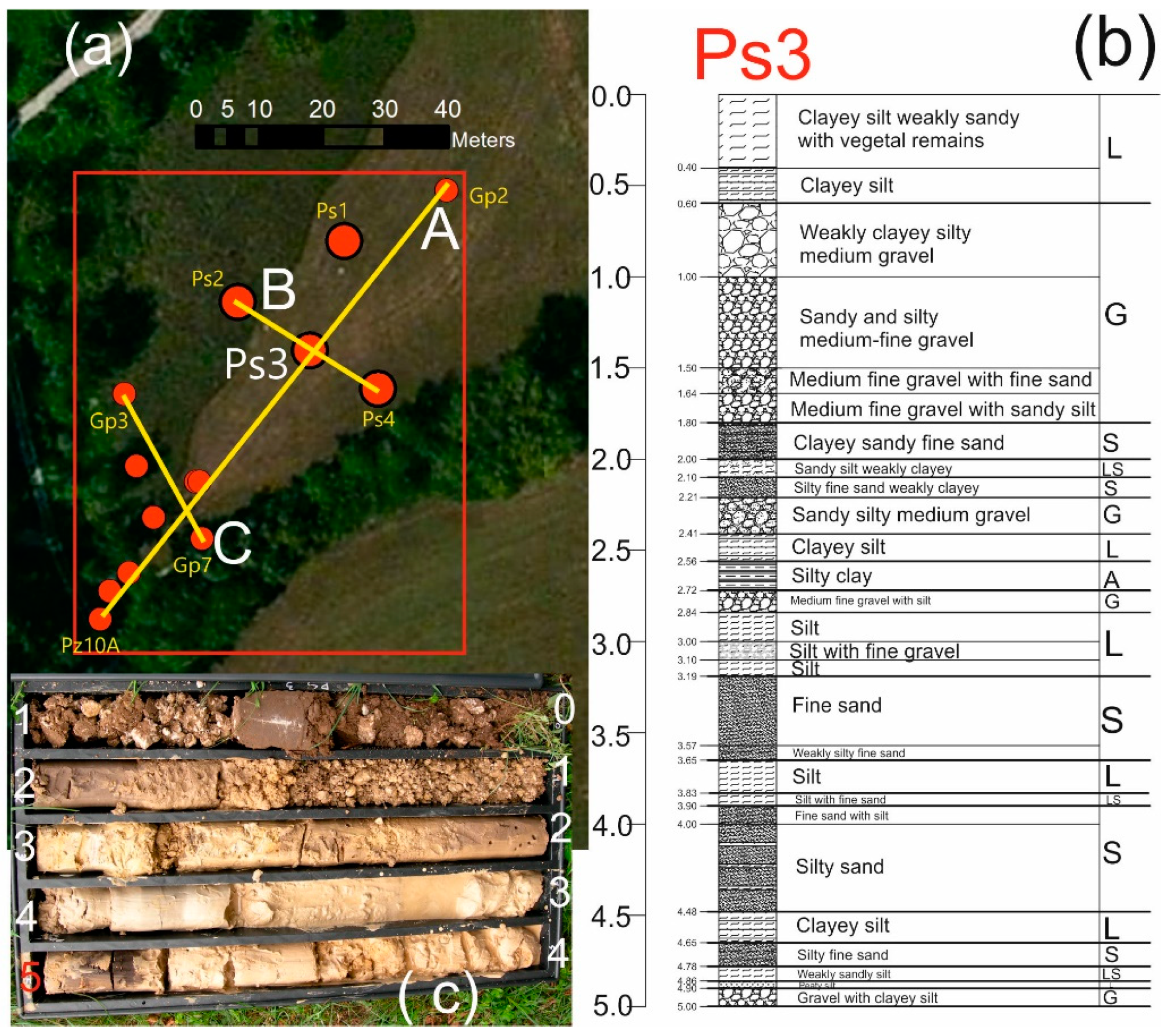
In the considered area (1.5 ha), 39 piezometers are present with a depth ranging from 1.6 to 22 m and a diameter ranging from 50 to 90 mm. The structural characteristics of 29 piezometers are available. The subsurface composition, and consequently the hydrogeological features, show high heterogeneity with gravel horizons alternating with sandy, silty and clayey levels (Figure 2b,c). The shallow unconfined aquifer of this area is essentially recharged by rainfall [53,54].
Figure 2a shows the red rectangle of the simulation area with the location of 13 available borehole logs that are 5 m deep and have data every 2 cm. An example of stratigraphy (Ps3) is given in Figure 2b.
Markovian Categorical Prediction (MCP)
Traditionally, Markov chains are stochastic processes described by a probabilistic model along a single dimension (usually time) subdivided into discrete lags. The extension of this concept arises by the definition of a Markov process involving continuous lags in a d dimensional space [21].
By considering a stationary process, the transition probability between two lithologies (categories), i and j, in two locations, s and s + h, is defined as:
where K is the total number of lithologies (1,…, K) that the categorical random variable Z can assume as outcomes and h is a multidimensional lag from any observed location s. The transition probability is the element in the i-th row and in the j-th column of the matrix T(h) such that:
where the transition rate matrix depends both on the length of the lag h and its direction.
Carle and Fogg, 1997, formulated the transition rate matrix for the direction h by an ellipsoidal approximation, which combines the matrix derived from the main axial directions. The vector indicates the standard basis vector of dimension d, whose k-th component (corresponding to the k-th axial direction) is one and the others are zeros. Considering our scope, the first problem consists of the estimation of the transition rate matrix components , and the second arises from the choice of the conditional probability approximation adopted for simulating/predicting the lithologies. Different methods address the first problem and are implemented in spMC. These include the mean lengths and the maximum entropy method suggested by Carle and Fogg, 1997. The lithological simulation and prediction algorithms implemented in spMC are based on attempts proposed to solve the second problem, and consider different approximations of the conditional probability:
where denotes the simulation/prediction spatial location without lithological information, represents the l th spatial position of the available data, and corresponds to the observed lithology of the random variable .
The classical approximation of (3) is based on the cokriging or kriging approach, while other formulations bypass the kriging formalism and its related issues. For instance, Bogaert, 2002 introduced a Bayesian procedure that exploits the maximum entropy principle, but requires a computationally intensive entropy optimization. Allard et al., 2011, avoided the entropy optimization by aggregating the transition probabilities (Markovian-type Categorical Prediction (MCP)) to approximate the optimal solution of the maximum entropy approach. The approximation of the conditional probability proposed by Allard et al., 2011, is formulated as follow:
where denotes the proportion of the i-th lithology considered for the location , and is the transition probability to the i-th lithology in from the k-th lithology observed in the location .
The sources of uncertainty in a conditional simulation setting are mainly related to the several approximations used in the computation of the final conditional probability. The estimation process consists of several steps to compute transition rates along axial directions. These steps introduce variability in the estimates of the rates by aligning the data according to a reasonable angular tolerance, and a possible model misspecification due to the ellipsoidal approximation [21] along non-axial directions may reduce the precision of the transition probabilities. In addition, the approximation used to produce the conditional probabilities affects the accuracy of the resulting predicted lithologies. All these sources are considered together the intrinsic variability of the spatial random process, which increases as the distance between the prediction point, , and the data becomes wider.
To evaluate the uncertainties of the simulation process the standardized conditional entropy [55] is computed as:
This index allows to assess the spatial distribution of the simulations by highlighting areas that are more uncertain due to the lack of data. Other indexes, such as producer and user accuracies, can be used to assess the ability of the methodology in reproducing the correct lithology by using validation data; however, this type of analysis goes beyond the aims of this paper.
3. Data Analysis
As described in Section 2, 39 piezometers are present in an area of 1.5 ha, but only 13 are drilled in the simulated area (70 m x 60 m) (red box in Figure 2a).
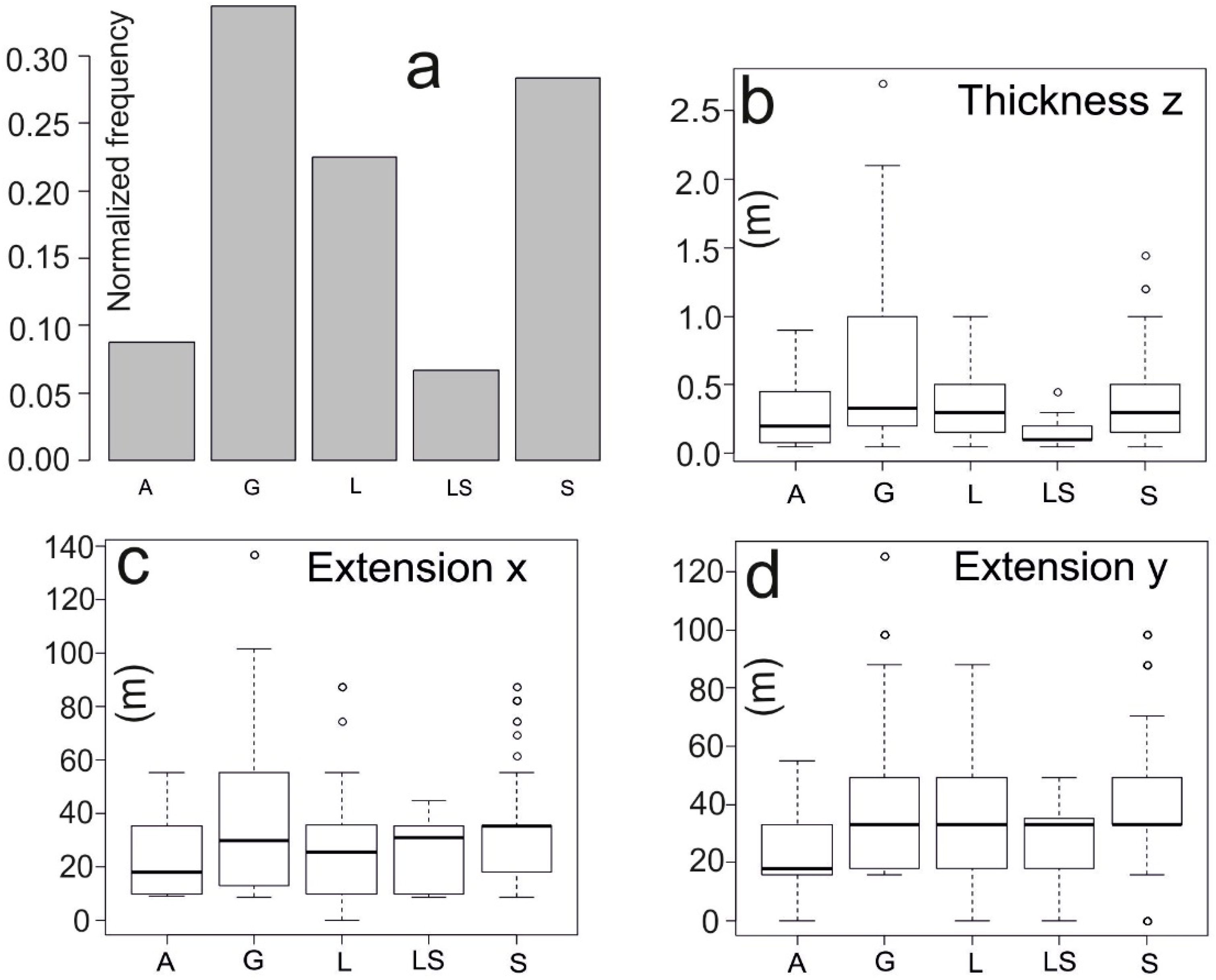
The first step simplifies the local complex heterogeneity of the available 13 stratigraphic logs into five lithologies: A = clay, G = gravel, L = silt, LS = silty sand and S = sand. All analyses are performed by the package spMC [44] implemented in R, which is a free software environment for statistical computing and graphics. Figure 3a shows the sediment distribution indicated in the subsoil G (0.34), S (0.28) and L (0.22) as more frequent than A (0.09) and LS (0.07). The boxplots of Figure 3b–d show the thickness/extension distribution of the lithologies along the directions Z (depth), X (longitude), and Y (latitude), and their mean values are exposed in Table 1. The horizontal extensions are based on the 13 borehole locations that are successively considered during the simulation (Figure 2a). The extensions in X and Y are calculated for all five lithologies through the mean lengths of spatial embedded Markov chains.
As visible in Figure 3b, layers made out of gravels (G) present more variation in thickness than the other four lithologies, while the variation in the lithological extension along the directions X and Y (Figure 3c,d) is higher but comparable between them.
The analysis of the embedded transition probabilities in 3D allows for a first rough juxtapositional investigation among the five considered materials, independently of their thickness or extension.
For instance, the analysis of Table 2 along the direction Z (depth) highlights that, among all the five lithologies, it is more probable to find a layer of sandy silt (LS) above a layer of sand (S) (0.62) than a layer of S above a layer of LS (0.36), while the probability to find a layer of gravel (G) above a layer of silt (L) (0.36) is similar to its opposite condition (0.37). It is also evident that the probabilities seeing a layer of sandy silt (LS) above a layer of clay (A) (0.07) or a layer of gravel (G) above a layer of sandy silt (LS) (0.11) are both low.
The analyses of Table 2 along the direction X (longitude) and Y (latitude) shows the estimated probability that one lithology laterally neighbors another. For instance, it is evident that there is a high probability to pass from clay (A) to gravel (G) (0.64 along direction X and 0.66 along Y). Moreover, similar probabilities to pass from L to G (0.70) and from G to L (0.69) have been computed along Y, while the probability to pass from A to LS is the smallest (0.00 along Y and 0.05 along X).
4. Transiogram Analysis
The lithological transition probabilities are analyzed along the directions Z (depth), X (longitude) and Y (latitude) in relation to different distances (h). These probabilities are modeled through continuous lag Markov chains and used in the next section for the lithological simulation.
The theoretical transition probabilities are calculated by estimating transition rates with a maximum entropy approach that uses the trimmed mean of the lithological layers.
The analysis of the diagonal transiogram (e.g., A vs. A, G vs. G, etc.) in Figure 4 gives some information about the thickness of the layers by showing the probabilities of finding the same lithologies juxtaposed every 5 cm in depth (direction Z). Along the diagonal of auto transitions, a high empirical probability is visible in sand (S), and it reaches a sill of about 0.4 at a range of 1 m (Figure 4a). At the same time, the empirical auto transition probability in gravel (G) regularly decreases in depth down to 0 (Figure 4b). This could mean that sandy layers are thinner (sand thickness 0.38 m) and more frequent than the gravely ones (gravel thickness 0.70 m). This is also visible in the boxplot of the length distribution for sand in Figure 3b. The transiogram behavior (Figure 4c) for silt (L) suggests that the thickness of silt layers is comparable to that of sand layers (S), but silty layers are more frequent than the sandy ones (compare Figure 4c vs. Figure 4a). The probabilities of auto transition for clay (A) and sandy silt (LS) (Figure 4d,e) quickly achieve a very low sill value. This makes it less likely to find thick or frequent layers for those two lithologies.
The off-diagonal transiogram analysis of Figure 4 gives some information about the juxtapositional tendency of the materials at different distances h. The results are comparable with those of embedded transition probability in Table 2, but, in this case, transition probabilities are plotted versus distances h. A high probability of finding sandy silt (LS) in contact with and above sand (S) with a sill of approximately 0.5 and a range of about 1 m (Figure 4f) is notable. A “hole effect” is also visible in the transition diagram from clay (A) above silt (L) (Figure 4g), but also from silt (A) above sand (S) (Figure 4h), indicating an irregular alternate occurrence in those two pairs of lithologies. Transiograms along the directions X and Y are calculated without considering Walther’s law of facies, stating that the vertical (along Z, i.e., depth) succession of facies reflects their lateral changes. This probably produces less interpretable experimental transiograms, but they are based on the information available from real data.
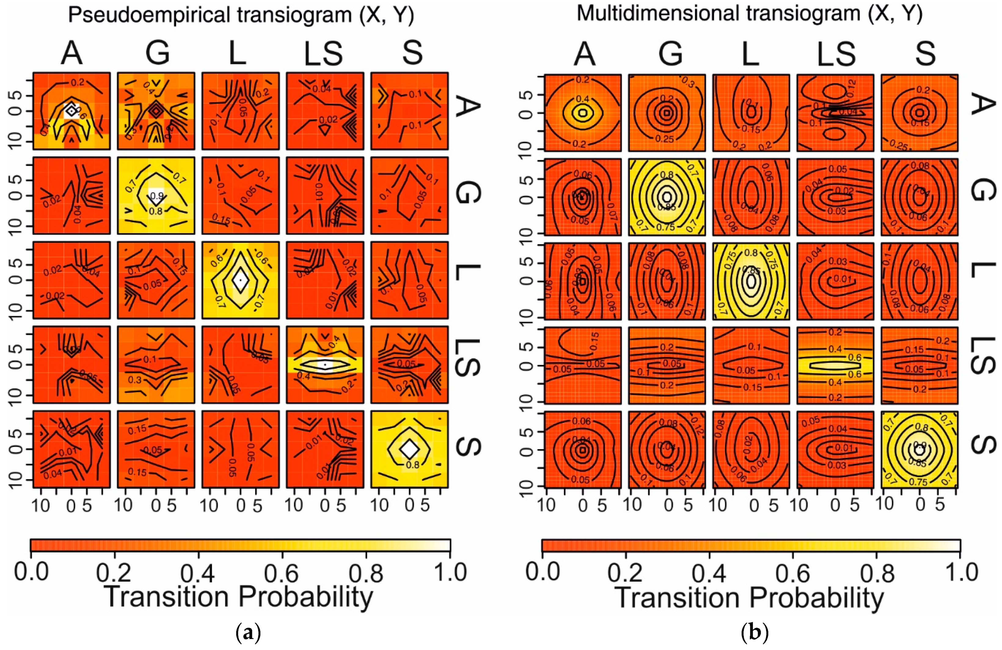
After analyzing the transiograms, the surface theoretical transiograms are studied with (Figure 5b) or without (Figure 5a) ellipsoidal interpolation calculated by experimental data. These diagrams highlight the anisotropies of the modeled transiograms in the X–Y plane.
The auto transition in silt (L) and gravel (G) show an anisotropy along the latitude. It is more probable to find silt and gravel along the Y direction (latitude) than the X direction (longitude). This is also confirmed from the lengths in Y and X (Table 1), while the visible anisotropy along X related to silty sand (LS) it is not visible in Table 1.
5. Simulation Results
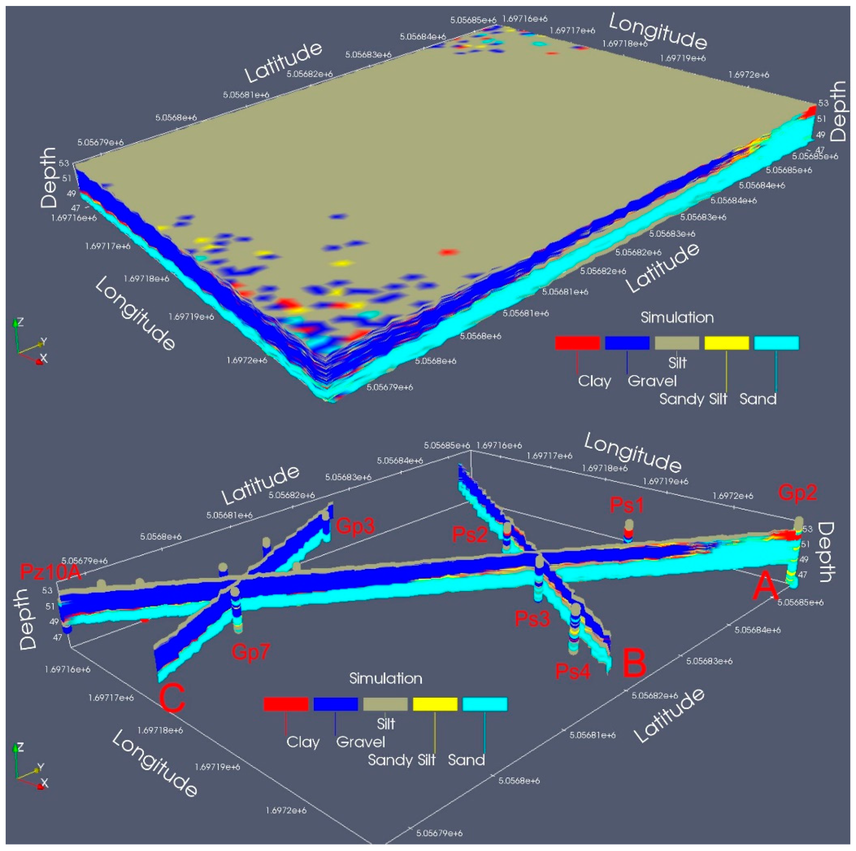
After the transiogram analysis and modeling, a 3D simulation of lithologies has been performed by means of the MCP algorithm. This algorithm is implemented in the spMC package and uses a maximum entropy approach in order to approximate the posterior conditional probabilities.
A small portion (70 × 60 × 5 m) of the hydrogeological zone described before has been converted into a discrete 3D grid of 56 × 69 × 91cells [1 × 1 × 0.05 m] (Figure 2).
An example of lithological heterogeneity in the studied area is visible in the core box of the 5 m deep borehole Ps3 exposed, also in Figure 2c. The aim of the geostatistical simulation performed by the MCP algorithm is to reproduce such a heterogeneity.
In Figure 6, the results of lithologic simulation are visible in 3D and in three cross-sections (A, B, C) from 48.5 to 53 m a.s.l., while the latitude and longitude are expressed according to the “Monte Mario Italy 1” coordinate system.
The simulation obtained by MCP algorithm is plotted through ParaView software [56]. ParaView is an open-source, multiplatform data analysis and visualization application.
The traces of those cross sections are also visible as yellow lines in Figure 2a. The first cross section (A) (Figure 6) is a diagonal obtained from the simulated area and starts from borehole Gp2 to Pz10A. The second (B) is almost perpendicular to the first one and passes through borehole Ps2 and Ps4. The third (C) passes through borehole Gp3 and Gp7.
The analysis of these simulated cross-sections confirms (compare Table 2, Figure 4f) as sandy silt (LS) layers are often located above sand (S) layers rather than vice versa. Moreover, sandy silt (L) layers are rarely below clay (A) layers as visible in Figure 4m and Table 2. A more probable situation occurs with regard to gravel (G) layers located below sandy silt (LS) layers, as shown in Figure 4n and Table 2.
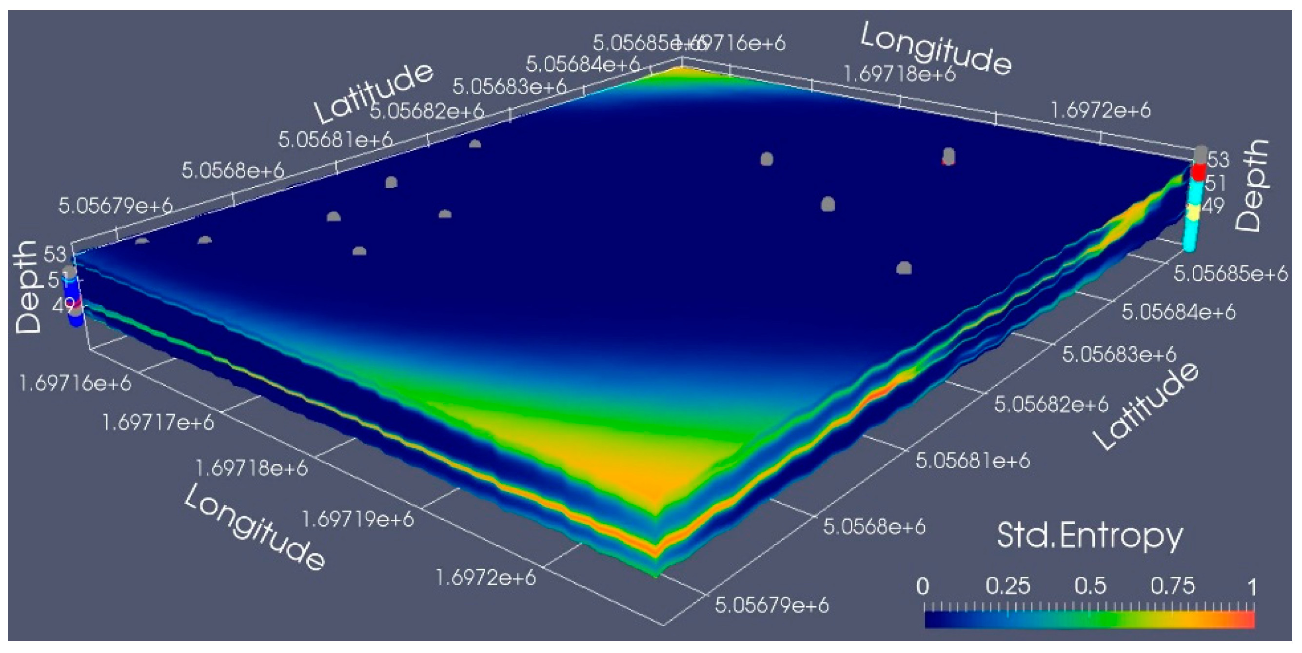
In this work, standardized conditional entropy index represents the uncertainty of the spatial information linked to the simulated lithologies. In other words, the 3D entropy index suggests both zones where the information is accurate and where lithological information should be improved. As is visible in Figure 7, the maximum entropy (i.e., entropy ≥ 0.9) is located in zones with a lack of boreholes. Low values of entropy, instead, cover the zones where more boreholes are located. The conditional entropy map depicts good reliability in the zones where the boreholes are present. More uncertain areas are located where the boreholes are missing or sparse. In this sense, the normalized entropy volume gives us an important hint for a possible enhancement of coring, showing where new information should be acquired (i.e., zones with entropy ≥ 0.9).
6. Conclusions
In this paper, a simulation of lithological distribution in a small area located in NE Italy has been carried out. Geostatistical reconstruction of subsoil, considering categorical data, is frequently made via the indicator kriging approach, which is affected by the aforementioned conceptual issues. Along these lines, a Markovian-type Categorical Prediction (MCP) implemented in the R package spMC has been applied to show the potentialities of the software and the advantages of this new geostatistical approach. The main results of that study pointed out some important aspects, both for application purposes and computational efficiency.
From a geological perspective, the pairwise comparison of juxtapositional tendencies of the lithologies (especially in depth), regardless of their distances, provides information on the depositional correlation among materials. This also explains the spatial changes of the probability in finding other materials. Furthermore, the inspection of the diagonal transiogram (i.e., autotransiograms) supplies the associated probability of finding lithological thickness. These two types of information play an important role for both the sedimentological and hydrogeological perspectives; in fact, one can infer depositional cycles and related hydrogeological structures that control flow direction. The MCP simulation reproduces the heterogeneity of the studied area well. This fact is also corroborated by the juxtaposition tendencies that are comparable with both the estimated Embedded Transition Probabilities (ETP) and transiogram results.
From a computational point of view, MCP simulates lithologies by using only the sums and products of univariate and bivariate probabilities. This approach is in agreement with the maximum entropy approach and produces consistent results with the lithological heterogeneity of the simulated area, by avoiding the well-known “order relation problem” of the indicator kriging. This simulation method avoids high computational burden, which is typical of the indicator kriging. HPC techniques further improve the computational efficiency and also allow us to increase the number of lithological categories considered during the simulation. In conclusion, the results obtained by the spMC package suggest that this software should be considered as a good candidate for simulating the subsoil lithological distributions of limited areas. Its computational capabilities and its efficacy in modeling heterogeneity allow for a wide application of spMC in hydrogeological modeling.
Author Contributions
Conceptualization, P.F.; methodology, C.G. and L.S.; software, L.S.; validation, P.F. and N.D.L.; writing—original draft preparation, P.F.; writing—review and editing, P.F., C.G., L.S., N.D.L. All authors have read and agree to the published version of the manuscript.
Funding
This research received no external funding.
Acknowledgments
The authors would like to thank the three anonymous reviewers of Hydrology for their many useful comments.
Conflicts of Interest
The authors declare no conflict of interest.
References
- Pyrcz, M.J.; Deutsch, C.V. Geostatistical Reservoir Modeling, 2nd ed.; Oxford University Press: Oxford, UK, 2014; p. 448. ISBN 978-0199731442. [Google Scholar]
- Koltermann, C.E.; Gorelick, S.M. Heterogeneity in sedimentary deposits: A review of structure-imitating, process-imitating, and descriptive approaches. Water Resour. Res. 1996, 32, 2617–2658. [Google Scholar] [CrossRef]
- De Marsily, G.; Delay, F.; Teles, V.; Schafmeister, M.T. Some current methods to represent the heterogeneity of natural media in hydrogeology. Hydrogeol. J. 1998, 6, 115–130. [Google Scholar] [CrossRef]
- De Marsily, G.; Delay, F.; Gonçalvès, J.; Renard, P.; Teles, V.; Violette, S. Dealing with spatial heterogeneity. Hydrogeol. J. 2005, 13, 161–183. [Google Scholar] [CrossRef]
- Al-Khalifa, M.A.; Payenberg, T.H.D.; Lang, S. Overcoming The Challenges of Building 3D Stochastic Reservoir Models Using Conceptual Geological Models: A Case Study. In Proceedings of the PE Middle East Oil and Gas Show and Conference, Manama, Bahrain, 11–14 March 2007; pp. 1–12. [Google Scholar]
- Comunian, A.; Renard, P.; Straubhaar, J.; Bayer, P. Three-dimensional high resolution fluvio-glacial aquifer analog—Part 2: Geostatistical modeling. J. Hydrol. 2011, 405, 10–23. [Google Scholar] [CrossRef] [Green Version]
- Dell’Arciprete, D.; Bersezio, R.; Felletti, F.; Giudici, M.; Comunian, A.; Renard, P. Comparison of three geostatistical methods for hydrofacies simulation: A test on alluvial sediments. Hydrogeol. J. 2012, 20, 299–311. [Google Scholar] [CrossRef]
- Marini, M.; Felletti, F.; Beretta, G.P.; Terrenghi, J. Three Geostatistical Methods for Hydrofacies Simulation Ranked Using a Large Borehole Lithology Dataset from the Venice Hinterland (NE Italy). Water 2018, 10, 844. [Google Scholar] [CrossRef] [Green Version]
- Haldorsen, H.H.; Chang, D.M. Notes on stochastic shales; from outcrop to simulation model. In Reservoir Characterization; Elsevier: Amsterdam, The Netherlands, 1986; pp. 445–485. [Google Scholar]
- Viseur, S. Stochastic Boolean Simulation of Fluvial Deposits: A New Approach Combining Accuracy with Efficiency. In Proceedings of the SPE Annual Technical Conference and Exhibition, Houston, TX, USA, 3–6 October 1999. [Google Scholar]
- Vargas-Guzmán, J.A.; Al-Qassab, H. Spatial conditional simulation of facies objects for modeling complex clastic reservoirs. J. Pet. Sci. Eng. 2006, 54, 1–9. [Google Scholar] [CrossRef]
- Matheron, G.; Beucher, H.; De Fouquet, C.; Galli, A.; Guerillot, D.; Ravenne, C. Conditional Simulation of the Geometry of Fluvio-Deltaic Reservoirs. In Proceedings of the SPE Annual Technical Conference and Exhibition, Dallas, TX, USA, 27–30 September 1987. [Google Scholar]
- Armstrong, M. Plurigaussian Simulations in Geosciences; Springer: Berlin/Heidelberg, Germany, 2011; ISBN 3642196071. [Google Scholar]
- Journel, A.G. Nonparametric estimation of spatial distributions. J. Int. Assoc. Math. Geol. 1983, 15, 445–468. [Google Scholar] [CrossRef]
- Trevisani, S.; Fabbri, P. Geostatistical modeling of a heterogeneous site bordering the Venice lagoon, Italy. Ground. Water 2010, 48, 614–623. [Google Scholar] [CrossRef]
- Dalla Libera, N.; Fabbri, P.; Mason, L.; Piccinini, L.; Pola, M. A local natural background level concept to improve the natural background level: A case study on the drainage basin of the Venetian Lagoon in Northeastern Italy. Environ. Earth Sci. 2018, 77, 487. [Google Scholar] [CrossRef]
- Fabbri, P. Probabilistic Assessment of Temperature in the Euganean Geothermal Area (Veneto Region, NE Italy). Math. Geol. 2001, 33, 745–760. [Google Scholar] [CrossRef]
- Schwarzacher, W. The use of Markov chains in the study of sedimentary cycles. J. Int. Assoc. Math. Geol. 1969, 1, 17–39. [Google Scholar] [CrossRef]
- Luo, J. Transition Probability Approach to Statistical Analysis of Spatial Qualitative Variables in Geology; Springer: Boston, MA, USA, 1996; pp. 281–299. [Google Scholar]
- Carle, S.F.; Fogg, G.E. Transition probability-based indicator geostatistics. Math. Geol. 1996, 28, 453–476. [Google Scholar] [CrossRef]
- Carle, S.F.; Fogg, G.E. Modeling Spatial Variability with One and Multidimensional Continuous-Lag Markov Chains. Math. Geol. 1997, 29, 891–918. [Google Scholar] [CrossRef]
- Lee, S.Y.; Carle, S.F.; Fogg, G.E. Geologic heterogeneity and a comparison of two geostatistical models: Sequential Gaussian and transition probability-based geostatistical simulation. Adv. Water Resour. 2007, 30, 1914–1932. [Google Scholar] [CrossRef]
- Weissmann, G.S.; Carle, S.F.; Fogg, G.E. Three-dimensional hydrofacies modeling based on soil surveys and transition probability geostatistics. Water Resour. Res. 1999, 35, 1761–1770. [Google Scholar] [CrossRef] [Green Version]
- Weissmann, G.S.; Fogg, G.E. Multi-scale alluvial fan heterogeneity modeled with transition probability geostatistics in a sequence stratigraphic framework. J. Hydrol. 1999, 226, 48–65. [Google Scholar] [CrossRef]
- Miall, A.D. Markov chain analysis applied to an ancient alluvial plain succession. Sedimentology 1973, 20, 347–364. [Google Scholar] [CrossRef]
- Hattori, I. Entropy in Markov chains and discrimination of cyclic patterns in lithologic successions. J. Int. Assoc. Math. Geol. 1976, 8, 477–497. [Google Scholar] [CrossRef]
- Jef Caers, T.Z. Multiple-point Geostatistics: A Quantitative Vehicle for Integrating Geologic Analogs into Multiple Reservoir Models. AAPG Memoir 2005, 383–394, ISSN: 02718529. [Google Scholar]
- Chugunova, T.L.; Hu, L.Y. Multiple-Point simulations constrained by continuous auxiliary data. Math. Geosci. 2008, 40, 133–146. [Google Scholar] [CrossRef]
- Comunian, A.; Renard, P.; Straubhaar, J. 3D multiple-point statistics simulation using 2D training images. Comput. Geosci. 2012, 40, 49–65. [Google Scholar] [CrossRef] [Green Version]
- Mariethoz, G.; Renard, P. Reconstruction of Incomplete Data Sets or Images Using Direct Sampling. Math. Geosci. 2010, 42, 245–268. [Google Scholar] [CrossRef] [Green Version]
- Strebelle, S. Conditional simulation of complex geological structures using multiple-point statistics. Math. Geol. 2002, 34, 1–21. [Google Scholar] [CrossRef]
- Emery, X.; Lantuéjoul, C. Can a Training Image Be a Substitute for a Random Field Model? Math. Geosci. 2014, 46, 133–147. [Google Scholar] [CrossRef]
- Breslow, N.E.; Clayton, D.G. Approximate Inference in Generalized Linear Mixed Models. J. Am. Stat. Assoc. 1993, 88, 9–25. [Google Scholar]
- Cao, G.; Kyriakidis, P.C.; Goodchild, M.F. A multinomial logistic mixed model for the prediction of categorical spatial data. Int. J. Geogr. Inf. Sci. 2011, 25, 2071–2086. [Google Scholar] [CrossRef]
- Csiszar, I. Why Least Squares and Maximum Entropy? An Axiomatic Approach to Inference for Linear Inverse Problems. Ann. Stat. 1991, 19, 2032–2066. [Google Scholar] [CrossRef]
- Christakos, G. A Bayesian/maximum-entropy view to the spatial estimation problem. Math. Geol. 1990, 22, 763–777. [Google Scholar] [CrossRef]
- Bogaert, P. Spatial prediction of categorical variables: The Bayesian maximum entropy approach. Stoch. Environ. Res. Risk Assess. 2002, 16, 425–448. [Google Scholar] [CrossRef]
- Bogaert, P.; D’Or, D. Estimating Soil Properties from Thematic Soil Maps. Soil Sci. Soc. Am. J. 2002, 66, 1492–1500. [Google Scholar] [CrossRef]
- D’Or, D.; Bogaert, P.; Christakos, G. Application of the BME approach to soil texture mapping. Stoch. Environ. Res. Risk Assess. 2001, 15, 87–100. [Google Scholar] [CrossRef]
- D’Or, D.; Bogaert, P. Spatial prediction of categorical variables with the Bayesian Maximum Entropy approach: The Ooypolder case study. Eur. J. Soil Sci. 2004, 55, 763–775. [Google Scholar] [CrossRef]
- Allard, D.; D’Or, D.; Froidevaux, R. An efficient maximum entropy approach for categorical variable prediction. Eur. J. Soil Sci. 2011, 62, 381–393. [Google Scholar] [CrossRef]
- Huang, X.; Wang, Z.; Guo, J. Prediction of categorical spatial data via Bayesian updating. Int. J. Geogr. Inf. Sci. 2016, 30, 1426–1449. [Google Scholar] [CrossRef]
- Allard, D.; Comunian, A.; Renard, P. Probability Aggregation Methods in Geoscience. Math. Geosci. 2012, 44, 545–581. [Google Scholar] [CrossRef]
- Sartore, L.; Fabbri, P.; Gaetan, C. spMC: An R-package for 3D lithological reconstructions based on spatial Markov chains. Comput. Geosci. 2016, 94, 40–47. [Google Scholar] [CrossRef] [Green Version]
- R Development Core Team. R: A Language and Environment for Statistical Computing; R Foundation for Statistical Computing: Vienna, Austria, 2019; Volume 2. [Google Scholar]
- De Supinski, B.; Klemm, M. OpenMP Technical Report 7: Version 5.0 Public Comment Draft EDITORS; Austin, TX 78746, USA. 2018. Available online: https://www.openmp.org/wp-content/uploads/openmp-TR7.pdf (accessed on 5 March 2020).
- Fontana, A.; Mozzi, P.; Bondesan, A. Alluvial megafans in the Venetian-Friulian Plain (north-eastern Italy): Evidence of sedimentary and erosive phases during Late Pleistocene and Holocene. Quat. Int. 2008, 189, 71–90. [Google Scholar] [CrossRef]
- Carraro, A.; Fabbri, P.; Giaretta, A.; Peruzzoa, L.; Tateo, F.; Tellini, F. Effects of redox conditions on the control of arsenic mobility in shallow alluvial aquifers on the Venetian Plain (italy). Sci. Total Environ. 2015, 532, 581–594. [Google Scholar] [CrossRef]
- Carraro, A.; Fabbri, P.; Giaretta, A.; Peruzzo, L.; Tateo, F.; Tellini, F. Arsenic anomalies in shallow Venetian Plain (Northeast Italy) groundwater. Environ. Earth Sci. 2013, 70, 3067–3084. [Google Scholar] [CrossRef]
- Fabbri, P.; Gaetan, C.; Zangheri, P. Transfer function-noise modelling of an aquifer system in NE Italy. Hydrol. Process. 2011, 25, 194–206. [Google Scholar] [CrossRef]
- Fabbri, P.; Piccinini, L. Assessing transmissivity from specific capacity in an alluvial aquifer in the middle Venetian plain (NE Italy). Water Sci. Technol. 2013, 67, 2000–2008. [Google Scholar] [CrossRef] [PubMed]
- Vorlicek, P.A.; Antonelli, R.; Fabbri, P.; Rausch, R. Quantitative hydrogeological studies of the Treviso alluvial plain, NE Italy. Q. J. Eng. Geol. Hydrogeol. 2004, 37, 23–29. [Google Scholar] [CrossRef]
- Fabbri, P.; Piccinini, L.; Marcolongo, E.; Pola, M.; Conchetto, E.; Zangheri, P. Does a change of irrigation technique impact on groundwater resources? A case study in Northeastern Italy. Environ. Sci. Policy 2016, 63, 63–75. [Google Scholar] [CrossRef]
- Fabbri, P.; Ortombina, M.; Piccinini, L. Estimation of Hydraulic Conductivity Using the Slug Test Method in a Shallow Aquifer in the Venetian Plain (NE, Italy). AQUA Mundi 2012, 3, 125–133. [Google Scholar]
- Journel, A.G.; Deutsch, C.V. Entropy and spatial disorder. Math. Geol. 1993, 25, 329–355. [Google Scholar] [CrossRef]
- Ahrens, J.; Geveci, B.; Law, C. ParaView: An End-User Tool for Large Data Visualization. In The Visualization Handbook; Academic Press: Cambridge, MA, USA, 2005; pp. 717–731. [Google Scholar] [CrossRef]
Figure 1.
Geographical location of studied area and cross section of Venetian Plain (Fabbri et al., 2011, modified). Map coordinates are shown in metric units, Monte Mario/Italy Zone 1.
Figure 1.
Geographical location of studied area and cross section of Venetian Plain (Fabbri et al., 2011, modified). Map coordinates are shown in metric units, Monte Mario/Italy Zone 1.

Figure 2.
(a) Location of 13 piezometers (red dots); simulated area (red rectangle); traces of cross sections (yellow lines) (image from Google Earth); (b) stratigraphy of Ps3 with example of lithologic reduction to 5 materials; (c) core box of Ps3 piezometer.
Figure 2.
(a) Location of 13 piezometers (red dots); simulated area (red rectangle); traces of cross sections (yellow lines) (image from Google Earth); (b) stratigraphy of Ps3 with example of lithologic reduction to 5 materials; (c) core box of Ps3 piezometer.

Figure 3.
Normalized frequency distribution of lithologies (a); boxplot thickness for every lithology along direction Z (depth) (b); extension of the lithologies along the directions X (c) and Y (d).
Figure 3.
Normalized frequency distribution of lithologies (a); boxplot thickness for every lithology along direction Z (depth) (b); extension of the lithologies along the directions X (c) and Y (d).

Figure 4.
Experimental transition probabilities with respect to the distance (h) (black circles) and theoretical transition probabilities modeled by Markov chains (red lines) along the directions Z, X and Y).
Figure 4.
Experimental transition probabilities with respect to the distance (h) (black circles) and theoretical transition probabilities modeled by Markov chains (red lines) along the directions Z, X and Y).

Figure 5.
Surface theoretical transiograms without (a) and with (b) ellipsoidal interpolation.

Figure 6.
Markovian-type Categorical Prediction (MCP) 3D simulation on 91 layers every 5 cm in depth from 53 to 48.5 m a.s.l.; cross sections A, B, C of MCP 3D simulation and simplified stratigraphies of the 13 boreholes.
Figure 6.
Markovian-type Categorical Prediction (MCP) 3D simulation on 91 layers every 5 cm in depth from 53 to 48.5 m a.s.l.; cross sections A, B, C of MCP 3D simulation and simplified stratigraphies of the 13 boreholes.

Figure 7.
Standardized conditional entropy index in the studied area.


Table 1.
Mean of thickness along Z, and its extension along the directions X and Y for the considered lithologies.
Table 1.
Mean of thickness along Z, and its extension along the directions X and Y for the considered lithologies.
| Lithology | Thickness Z (m) | Extension X (m) | Extension Y (m) |
|---|---|---|---|
| Clay (A) | 0.27 | 21.15 | 20.67 |
| Gravel (G) | 0.70 | 32.99 | 37.74 |
| Silt (L) | 0.35 | 26.55 | 33.13 |
| Silty Sand (LS) | 0.14 | 23.73 | 31.83 |
| Sand (S) | 0.38 | 31.31 | 37.33 |
Table 2.
Embedded Transition Probabilities (ETP) along the directions Z (depth), X (longitude) and Y (latitude).
Table 2.
Embedded Transition Probabilities (ETP) along the directions Z (depth), X (longitude) and Y (latitude).
| Z | A | G | L | LS | S | X | A | G | L | LS | S | Y | A | G | L | LS | S |
| A | - | 0.29 | 0.12 | 0.18 | 0.41 | A | - | 0.64 | 0.14 | 0.05 | 0.18 | A | - | 0.66 | 0.11 | 0.00 | 0.23 |
| G | 0.14 | - | 0.36 | 0.11 | 0.39 | G | 0.24 | - | 0.31 | 0.10 | 0.36 | G | 0.08 | - | 0.69 | 0.08 | 0.15 |
| L | 0.14 | 0.37 | - | 0.20 | 0.26 | L | 0.20 | 0.40 | - | 0.10 | 0.30 | L | 0.08 | 0.70 | - | 0.00 | 0.23 |
| LS | 0.07 | 0.14 | 0.17 | - | 0.62 | LS | 0.11 | 0.47 | 0.09 | - | 0.34 | LS | 0.06 | 0.47 | 0.26 | - | 0.21 |
| S | 0.20 | 0.18 | 0.23 | 0.36 | - | S | 0.04 | 0.45 | 0.41 | 0.10 | - | S | 0.15 | 0.42 | 0.40 | 0.03 | - |
© 2020 by the authors. Licensee MDPI, Basel, Switzerland. This article is an open access article distributed under the terms and conditions of the Creative Commons Attribution (CC BY) license (http://creativecommons.org/licenses/by/4.0/).
Share and Cite
MDPI and ACS Style
Fabbri, P.; Gaetan, C.; Sartore, L.; Dalla Libera, N. Subsoil Reconstruction in Geostatistics beyond Kriging: A Case Study in Veneto (NE Italy). Hydrology 2020, 7, 15. https://doi.org/10.3390/hydrology7010015
AMA Style
Fabbri P, Gaetan C, Sartore L, Dalla Libera N. Subsoil Reconstruction in Geostatistics beyond Kriging: A Case Study in Veneto (NE Italy). Hydrology. 2020; 7(1):15. https://doi.org/10.3390/hydrology7010015
Chicago/Turabian StyleFabbri, Paolo, Carlo Gaetan, Luca Sartore, and Nico Dalla Libera. 2020. "Subsoil Reconstruction in Geostatistics beyond Kriging: A Case Study in Veneto (NE Italy)" Hydrology 7, no. 1: 15. https://doi.org/10.3390/hydrology7010015
Note that from the first issue of 2016, this journal uses article numbers instead of page numbers. See further details here.