
A Survey on Text Classification Algorithms: From Text to Predictions


1
Department of Management, Ca’ Foscari University, 30123 Venice, Italy
2
Department of Environmental Sciences, Informatics and Statistics, Ca’ Foscari University, 30123 Venice, Italy
*
Author to whom correspondence should be addressed.
Information 2022, 13(2), 83; https://doi.org/10.3390/info13020083
Submission received: 10 January 2022
/
Revised: 28 January 2022
/
Accepted: 9 February 2022
/
Published: 11 February 2022
(This article belongs to the Topic Big Data and Artificial Intelligence)
Abstract
:In recent years, the exponential growth of digital documents has been met by rapid progress in text classification techniques. Newly proposed machine learning algorithms leverage the latest advancements in deep learning methods, allowing for the automatic extraction of expressive features. The swift development of these methods has led to a plethora of strategies to encode natural language into machine-interpretable data. The latest language modelling algorithms are used in conjunction with ad hoc preprocessing procedures, of which the description is often omitted in favour of a more detailed explanation of the classification step. This paper offers a concise review of recent text classification models, with emphasis on the flow of data, from raw text to output labels. We highlight the differences between earlier methods and more recent, deep learning-based methods in both their functioning and in how they transform input data. To give a better perspective on the text classification landscape, we provide an overview of datasets for the English language, as well as supplying instructions for the synthesis of two new multilabel datasets, which we found to be particularly scarce in this setting. Finally, we provide an outline of new experimental results and discuss the open research challenges posed by deep learning-based language models.
1. Introduction
Text classification (TC) is a task of fundamental importance, and it has been gaining traction thanks to recent developments in the fields of text mining and natural language processing (NLP). Text classification methods share the common goal of designating a predefined label for a given input text, though this denomination can refer to a variety of specialised methods applied to different domains.
Classic examples of TC include information retrieval, topic labelling, sentiment analysis, and news classification. However, TC has practical applications that extend beyond simple categorisation, such as extractive question answering and summarisation systems. In this case, the intuitive notion of “label” is substituted with a choice between candidates (e.g., an answer or a sentence to include in a summary).
The speed at which textual information is currently being created has long outclassed manual solutions to these tasks, meaning that TC methods are not only useful, but also strictly necessary. Accordingly, developing accurate and unbiased TC systems is of paramount importance.
1.1. Text Classification Tasks
A variety of standard definitions for TC tasks exist in the NLP research area, often used as benchmarks to evaluate new methods. We outline the main representatives, approximately following the taxonomy proposed by Li et al. [1]:
- •
- Sentiment analysis (SA): the task of understanding affective states and subjective information contained in a piece of text, often categorised in terms of stirred emotions;
- •
- Topic labelling (TL): the task of recognising one or more themes for a piece of text (i.e., its topics);
- •
- News classification (NC): the task of assigning categories to news pieces, such as topics or user interests;
- •
- Question answering (QA): the task of selecting an answer to a question, selecting from potential candidate sentences (usually extracted from a context document). This task is usually framed as binary or multiclass classification;
- •
- Natural language inference (NLI): the task of determining whether two sentences entail one another (classifying if the entailment occurs in one of the two directions, or neither);
- •
- Named entity recognition (NER): the task of locating named entities within unstructured text, labelling them with predefined categories;
- •
- Syntactic parsing (SP): a series of tasks related to predicting morpho-syntactic properties of words, such as part-of-speech (PoS) tagging, speech dependencies and semantic role labelling.
It is worth noting that these are generic formulations, meaning that specific tasks will present themselves with slight differences as contextualized to a specific domain.
1.2. Text Representation
An important step required by any TC procedure is the projection of text features in a chosen feature space. Because of its lack of structure (from a computational point of view), it is necessary to apply a number of operations, in order to gradually transform it into a form that is digestible for a computer. Preprocessing must be mindful of the models that are intended to be used in the later stages of the classification pipeline, since there is no “silver bullet” solution.
Most notably, earlier methods rely heavily on a manual feature engineering step, which necessitates considerate treatment and domain expertise. Later methods based on deep learning, on the other hand, are notably different because of the automatic extraction of features. As we will explore, preprocessing is still important for these methods, though it may be applied differently because of the assumptions that they make.
1.3. Broad Categorization of Text Classification Methods
In this work, machine learning methods are divided into the two broad categories of “shallow” and “deep” approaches, which we proceed to define.
1.3.1. Shallow Learning Approaches
Earlier methods are frequently defined as “shallow learning” approaches. However, since this definition is not one that is particularly standardised or agreed upon, we clarify that, with this term, we refer to all those traditional or classical methods related to conventional machine learning. That is, this group encompasses all of those methods preceding neural networks of which the prediction is based on hand-engineered features. In addition, this category also includes neural networks with very few (0–2) hidden layers, which are themselves referred to as “shallow” and which bridge the gap between this group of methods and their deep learning-based successors.
Shallow learning approaches are the successors of rule-based approaches, which they surpassed in both accuracy and stability. Shallow learning methods are still popular in many practical contexts, or as strong baselines. While they do not scale well to large amounts of data, they shine when resources are too scarce for deep methods to be effective. These classical approaches require a feature engineering step that may be costly, depending on the complexity of the domain. While the computational side of this cost can be significant, the domain knowledge requirements that are necessary for the correct application of appropriate feature extraction techniques may be more difficult to achieve in practice.
1.3.2. Deep Learning Approaches
The advent of deep learning models has affected all fields of artificial intelligence, including text classification. These methods have gained traction because of their ability to model complex features without the necessity of hand engineering them, removing part of the domain knowledge requirement. Instead, work has gone towards the development of neural network architectures able to extract effective representations for textual units. Recent developments have been particularly successful in this, giving birth to semantically meaningful and contextual representations. Automatic feature extraction is particularly advantageous in modelling textual data, as it is capable of leveraging the underlying linguistic structure of a document. This structure is intuitive to us if we understand the language, but is usually incomprehensible to a machine.
1.4. Major Differences and Contributions
Recent publications have explored text classification methods from a generic perspective. Among them, we cite the work by Li et al. [1], which provides a complete investigation of models, ranging from shallow to deep. Kowsari et al.’s [2] survey provides an excellent exploration of preprocessing steps, such as feature extraction and dimensionality reduction. Minaee et al.’s [3] work, on the other hand, focuses solely on a thorough exploration of deep approaches, though it also provides quantitative results for classical methods in its experimental performance analysis.
This work aims to enrich the landscape of text classification surveys by giving an outlook of each step involved in the development of a classifier for textual data. Therefore, we provide a detailed description of the most important data preparation operations utilised in conjunction with text classification algorithms. These passages of the TC pipeline are often overlooked, yet understanding their usage and the motivation behind their choices can prove fundamental in building an effective framework for this task. We continue by summarising information about primary English TC datasets and a general benchmark of state-of-the-art approaches in various sub-tasks. Moreover, we provide results on two newly synthesized multilabel TC datasets, laying out the process to reproduce them. We believe this to be an important contribution, as the sub-tasks that they address (namely multilabel TL and NC) are underrepresented.
In summary, this study’s main contributions are as follows:
- •
- We present an analysis of TC procedures, with emphasis on each step of the TC pipeline;
- •
- We showcase a variety of datasets in English, and provide the code for synthesising two multilabel classification datasets;
- •
- We present an overview of quantitative results for main methods in the literature, as well as for the datasets that we presented, complete with an analysis of evaluation metrics.
The rest of the survey is organised as follows. Section 2 explores preprocessing operations in TC pipelines, going through standard operations as well as common tokenisation strategies for more recent, deep learning-based models. Section 3 describes methodologies utilised to project preprocessed data into feature space, starting again from earlier approaches, while also describing word embeddings based on shallow neural networks. Section 4 gives a brief overview of generic classifiers commonly used with such features, while Section 5 goes more in depth into explaining the current landscape of deep learning-based classification methods. We move towards the experimental part of the survey in Section 6, showcasing prominent datasets (as well as two newly synthesised ones) and quantitative results. Finally, we discuss future research directions in Section 7 and conclude in Section 8.
Code and datasets used for experiments in this work are published and available (when legally possible) at https://gitlab.com/distration/dsi-nlp-publib (accessed on 28 December 2021).
2. Preprocessing
Input data for natural language tasks like TC consist of raw, unstructured text. Textual information, unlike other types of data such as images or temporal series, does not possess an intrinsic numerical representation; before feeding it to any classifier, then, it must be projected into an appropriate feature space. Preprocessing procedures are therefore of particular importance, as without them, there is no foundation for feature extraction procedures nor classification algorithms.
In this section, we will provide an overview of the preprocessing operations frequently utilised in TC methods. In the first part, we will cover standard methodologies, most frequently utilised in preparation of manual feature extraction techniques (which are explained in Section 3). We instead reserve the second part of this section to preprocessing operations as contextualized to deep models. By providing an overview of these approaches, we aim to highlight differences and innovations utilised by more recent models, thus offering a more thorough and transparent outlook on how textual data representation is done by state-of-the-art approaches.
2.1. Standard Preprocessing Operations
Preprocessing operations clean and normalise input data in order to improve the results of the feature extraction stage, regardless of whether it is manually built (in earlier methods) or automatically learnt (in deep learning methods). In this section, we outline the most prominent preprocessing techniques.
2.1.1. Tokenisation
The most basic preprocessing operation that must be applied to text is that of tokenisation. This procedure is what determines the level of granularity at which we analyse and generate textual data, and may be generally described as the process of breaking a stream of text into smaller chunks (historically called tokens). Until recently, most NLP models have utilised words as their atomic unit of choice, but recent approaches have been decomposing text into smaller units (such as character n-grams or even more maximal forms of decomposition, such as underlying bytes [4]).
Tokenisation [5], while often taken for granted, is a complex matter in itself and has been widely researched. Conventional methods are rule-based, and may be as simple as separating by space, punctuation and contractions. Clearly, much more refined knowledge-based approaches have been developed, still based on linguistic concepts. However, recent developments have moved strongly in the direction of data-driven tokenisers, which yield better results, but in which tokens no longer correspond to the traditional definition of a typographic unit. In other words, the modern meaning of “tokenisation” refers to the task of segmenting a sentence into units that, crucially, do not have a linguistic motivation or explanation. Because some of these methods still utilise traditional tokenisers as an initial step, conventional approaches are now often called “pre-tokenisers”.
An in-depth exploration of this topic is outside the scope of this survey, and we point to Mielke et al.’s work [6] for an excellent historical review of the evolution of tokenisers over recent years. As both tokenisation and classification approaches evolved in parallel, it is more common to associate conventional methods with pre-tokenisers. On the other hand, deep learning methods tend to approach tokenisation with the more recent and sophisticated methods, as will be outlined in Section 2.2.
2.1.2. Stopword and Noise Removal
The set of tokens produced by the tokenisation procedure may contain unnecessary or misleading elements. Textual noise such as special characters or superfluous symbols should be removed. It can be useful to remove stopwords [7], i.e., non-informative words that appear in large numbers but carry no semantic importance. Other normalisation procedures, such as lowercasing, misspelling correction, and the standardisation of slang words and abbreviations, may be useful in reducing the number of different elements in the feature space.
These processes, however, may cause interpretation issues (e.g., in English, “US” could be used as an acronym for the “United States”, but lowercasing would make it indistinguishable from “us” as a pronoun) [2]. Furthermore, the removal of stopwords and other pieces of text can be detrimental to more recent approaches. Deep models are trained to understand natural language; elements that constitute the syntax of a sentence may be fundamental to the model for it to understand the context of a piece of text. As such, destructive operations should not be applied indiscriminately.
2.1.3. Further Standardisation of Text
On the other hand, classical approaches may benefit from a further simplification of the feature space. Such methods are unable to capture significant semantic information about words; two inflections of the same word, then, cannot be distinguished (e.g., child vs. children), and will be treated as completely different pieces of information. Because of this, simplifying words by reducing inflections to a common form may be beneficial. This is achieved through the process of stemming (deriving a root form for a word) [8] or lemmatisation (deriving the lemma/canonical form for a word) [9]. These procedures can improve the performance of the overall classification, but at the same time, are not devoid of issues. Most notably, words with different meanings might have the same root or lemma, and these approaches will make them indistinguishable.
There are other useful operations that could help towards the improvement of a TC algorithm. An example of this is part-of-speech tagging; a “part of speech” is a category of words with similar grammatical properties, such as noun, verb, and adjective. This is sometimes included as a preprocessing step whenever the task could benefit from limiting the vocabulary to one or a subset of these parts of speech (for example, one might be interested in only nouns and adjectives). PoS tagging is a classification task in itself, and it is easy to recognise how misclassifications can result in worse overall performance by the models employing this procedure. An error of this kind can either introduce unwanted words or seclude important ones by mistake.
2.2. Preprocessing for Deep Models
As briefly mentioned, preprocessing operations should not be applied without consideration of the method being used. Recent models based on deep neural network architectures usually include similar steps for removing special characters, lowercasing and stripping letters of accents and apostrophes. Additionally, tokenised documents are also truncated or padded to a specified number of tokens to ensure that the model receives input samples of uniform size (i.e., with the same number of tokens).
Most of the attention, however, is shifted towards the effective tokenisation of text. Modern tokenisation approaches must strike a balance between a sufficiently large and expressive vocabulary and one that is too expensive in terms of memory. Therefore, different approaches have been proposed, of which we highlight the most prominent. As a side note, it is fairly common for modern tokenisers to also apply normalisation operations within their procedures [6].
2.2.1. Tokenisation in Deep Models
Deep models learn a vectorial representation for each token seen in training data. Learnt vectors are stored inside an embedding matrix, a data structure that maps recognised vocabulary terms to corresponding embeddings. The matrix size is hence dependent on the number of vocabulary terms and the embedding dimensionality. As mentioned, limited time and available memory imply the inability to deal with arbitrarily large vocabularies. These considerations motivate the development of different tokenisation techniques aimed at reducing the vocabulary size, minimising, at the same time, the number of unrepresented words. The latter are denoted as out-of-vocabulary (OOV) words, and are the central weakness of word-level models; these lead to unknown tokens at test time, which are not acceptable for most NLP tasks.
In pre-tokenisers, due to the fact that a representation is learnt for every word in the training corpus, related words like derivations and inflections (e.g., “snowboarding” and “snowboard”) are considered distinct, forcing the model to learn redundant encodings for each of them. Considering that the number of learnable parameters of such models is linearly dependent on the number of distinct words in the corpus, this issue may lead to unmanageable space and time requirements. Conversely, character-level tokenisation would imply a vocabulary set composed of all single characters in the corpus; this results in a minimal vocabulary, at least for alphabetical languages. While this strategy reduces memory and time complexity with respect to word-level tokenisation, it makes it much harder for the model to learn meaningful token representations. For instance, it is much harder to learn meaningful representation for the character “s” than it is for the word “snow”.
Since both of these simple strategies are not entirely satisfactory, most models employ hybrid techniques that segment words in sub-words. The general principle is that frequently used words should not be split into smaller words, but rare words should be decomposed into more meaningful segments. Table 1 summarises the main features of tokenisers commonly paired with deep neural models, which are presented in the next sections.
2.2.2. Byte Pair Encoding
The strategy that is now considered the breakthrough for sub-word tokenisation is Byte Pair Encoding (BPE). Originally proposed as a data compression algorithm [10], it was later adapted for sub-word segmentation (e.g., segmenting “snowboarding” as “snow”-“board”-“ing”) [11]. When learning a tokenisation, this algorithm iteratively computes the occurrences of consecutive pairs of vocabulary terms and merges the most frequent one into a new vocabulary word. When presented with unseen text to tokenise, the same merging procedure is performed by executing all recorded merges in the order in which they were performed during training. BPE’s vocabulary is initialised with the set of characters that appears in the training corpus.
A recent variation of this strategy is used with the GPT-2 [12] and RoBERTa [13] language models (see Section 5.4.4). In particular, these models utilise byte-level BPE [14], which applies this procedure to raw bytes rather than characters.
2.2.3. WordPiece
The WordPiece tokeniser [15], initially devised as a solution to Japanese text segmentation problems, implements a data-driven approach for splitting words into sub-words. It relies on the creation of n-gram-based language models (see Section 3.2) to recognise recurring syllables, prefixes and word segments in a corpus. Referring to the previous “snowboarding” example, the tokeniser must learn that “-ing” is a common ending for verbs, and a word should be likely split before and not after it. Hence, the goal of the model is the creation of a vocabulary of sub-words, such that the size of the training corpus is minimal when segmented according to the selected vocabulary. A greedy algorithm is used to solve this optimisation problem. Again, the initial vocabulary is composed of all single characters appearing in the input documents. Every successive iteration increases the vocabulary size by one, selecting the pair of sub-words that maximises the language model likelihood (hence the greedy nature) and merging them into a new vocabulary term.
The algorithm is stopped when the expected likelihood given by merging falls below a predefined threshold, or the maximum vocabulary size is reached. Recent approaches such as BERT [16] use tokenisers based on WordPiece; BERT, in particular, utilises a vocabulary of 30,000 tokens calibrated on English text.
2.2.4. UnigramLM
Similar to WordPiece, UnigramLM [17] is also based on the usage of language models to judge sub-word candidates (the name is derived from the fact that it utilises a simple unigram LM). Differently from Wordpiece, however, UnigramLM goes in the opposite direction, by initialising to a vocabulary size that is much larger than the count of sub-words desired (such as all pre-tokenised words and common sub-strings), and proceeds to iteratively remove them. In every iteration, the expectation–maximization algorithm is used to prune the lowest probability items, cycling until the vocabulary has reached the desired size.
Most interestingly, this sort of probabilistic setup results in different possible segmentations, all of which are consistent with the given strings. While the algorithm chooses the most likely segmentation in practice, it allows a sampling of different tokenisations based on their probabilities (which are recorded during training), allowing for what is defined as “sub-word regularisation”, which has been shown to improve results on some tasks. While UnigramLM is not commonly utilised by itself, it has seen use as a component of SentencePiece, which we now describe.
2.2.5. SentencePiece
Kudo and Richardson [18] propose some improvements over the previously described algorithms in a software package called SentencePiece, which contains optimised versions of the above approaches (though it is often mistakenly assumed to be a separate algorithm). In particular, all the tokenisers described so far depend on knowing which characters act as word separators in the corpus; these characters can be language-dependent, and specific pre-tokenisation procedures can be used to create rules for recognising word boundaries. SentencePiece removes the dependence on this step by considering text as a raw stream of characters, including word separators. Additionally, it implements sub-word regularisation techniques, mainly to improve segmentation for machine translation tasks. XLNet [19] and XLM-R [20] use SentencePiece to tokenise input data.
3. Projecting into Feature Space
Generally speaking, preprocessing pipelines transform bodies of text into lists of separated, standardised tokens. From a technical perspective, words are mapped to an index-based vocabulary, such as to simplify the internal representation of the tokens. However, tokens (or their index) must still be represented in a form that is digestible by a machine, i.e., a vectorial form. Many have been proposed over the years; this section provides an overview of the most popular and effective ones.
3.1. Bag-of-Words
The most intuitive representation can be found in the bag-of-words (BoW). This approach simplifies bodies of text by considering them as unordered collections of words. Clearly, this has the disadvantage of ignoring sentence structure and semantic relationships between sentence elements (as if shuffled inside of a “bag” of words). Nonetheless, despite its strong assumptions, it has been shown to obtain good results and has seen wide use. In general, efficient feature extraction can usually lead to strong performances, even when discarding important but difficult to encapsulate information, which is why this approach has been utilised extensively in NLP as well as other machine learning fields (where it is referred to as “bag-of-features”) [21,22,23].
The original idea behind BoW models is to represent each word as a one-hot-encoded vector with the same size as the vocabulary. It is immediate to see that this may lead to size issues, since the vocabulary itself may have a cardinality in the order of millions. As such, BoW models are usually implemented in conjunction with feature extraction techniques based on the multiplicity of words, which allows one to maintain a single vector per document rather than one for each word. For this purpose, term frequency (TF) counts the number of times that a word occurs within a body of text. When applied to a corpus of texts, rather than the explicit count, it is common practice to utilise the relative frequency of a term in the text in relation to other documents. One may also observe that, in very large corpora, common words, in particular, are inherently less useful (as they appear in all documents, hence do not help in distinguishing them). Consequently, TF is often weighted by inverse document frequency (IDF) [24], which lessens the effect of common words by penalising their overall score (and boosting the one of rarer words).
Depending on the size of the vocabulary, the size of TF-IDF representations may still be excessively large. To alleviate issues related to time complexity and memory consumption, it is possible to set a limit to the maximum number of features in the vectors (effectively pruning low-score words from the vocabulary). Alternatively, it is also possible to utilise a dimensionality reduction algorithm on the full-sized representations. Although a detailed description is outside the scope of this review, the general aim of these algorithms is to find a mapping between these representations and a lower-dimensional, compressed feature space. Popular methods include Principal Components Analysis (PCA) [25], Linear Discriminant Analysis (LDA) [26], and non-negative matrix factorization (NMF) [27]. See Kowsari et al.’s [2] survey for an introduction of these methods.
3.2. Language Models
Language modelling is the task of predicting the likelihood of a string given a sequence of preceding or surrounding context words—at its simplest, guess the next word in a sentence. Language models play an important part in more recent, deep learning-based developments, but their inception much precedes neural networks. N-gram models [28] are some of the earliest implementations of language models, and work by assigning probabilities to sequences of words (i.e., sentences). The specific interpretation of this probability value is task-dependent; intuitively, a higher score is associated with a better-structured sentence (e.g., a good translation).
While the goal is to assign probabilities to whole sentences, the task is related to the computation of the probability of an upcoming word, and is framed as such. These models usually make a simplifying assumption (the Markov assumption): it is assumed that the probability of an upcoming word only depends on the last n words before it. The probability value itself can be computed with methods such as Maximum Likelihood Estimation (MLE) [29], a robust estimation approach used thoroughly in probabilistic approaches. Notably, the BoW model can be seen as an n-Gram model with .
3.3. Word Embeddings
While previous methods have focused on capturing the syntactic representations of words and, in some cases, a small subset of the syntactic relationships that tie them together in sentences, they critically still lack the capability of capturing their semantic meaning. A classic example of this issue is represented by word synonyms; though they are—semantically speaking—the same, these models cannot capture their similarity. When looking at the feature space, this translates into representations that are orthogonal to each other, meaning that they are seen as completely different and separate.
In the last decade, researchers have proposed word embeddings as a solution to this problem. Intuitively, this self-supervised feature learning technique is aimed at learning a mapping between each piece of text (most commonly words, hence the name) to a n-dimensional vector of real numbers. An embedding is therefore a vectorial representation, which is digestible by a machine, but also encodes part of the underlying meaning of the words. These approaches are based on neural networks, which learn these mappings through different learning procedures; in general, they are based on the assumption that a word’s meaning can be extracted from its surrounding words in a sentence (similarly to language modelling, but focused on the embeddings as individual entities).
Earlier word embeddings are often informally defined as “static”, which can be attributed to how, in their basic form, they encode words outside of context. Practically speaking, this means that they do not model polysemy [30] (where an individual word can have different meanings). The embedding for a word is just one, regardless of how many meanings it could have; if a word token is particularly polysemous, it is likely that its embedding will be a combination of its multiple senses.
As an example, consider the word “sound”; as a noun, we may associate this with something that can be heard, whereas, as an adjective, we can associate it with a description of something in good condition. However, these are just two of the almost 50 different meanings that this word can have; based on this consideration, it appears obvious that a single representation can hardly be effective at representing them all at once. As will be further discussed in Section 5.4.7, recent developments have proposed to utilise surrounding context words in order to differentiate a word’s meaning.
3.3.1. Word2Vec
One of the first popular families of word embedding architectures is to be attributed to Mikolov et al.’s Word2Vec [31,32]. Their approach utilises shallow neural networks in order to create a high dimensional vector for each word (though they are much smaller and denser than, for example, TF-IDF vectors). Word2Vec was first proposed with two architectural variants: the Continuous-bag-of-words (CBOW) and the continuous skip-gram.
The way in which the CBOW approach learns word representations is to try to predict a middle word based on its surrounding context words. The reference to bag-of-words derives from the fact that the order of the context elements is not actually taken into account. The continuous skip-gram model instead flips the task on its head, as it attempts to predict the neighbours of a word, given the word itself.
These tasks are clearly hard, and the model is not meant to learn perfectly how to guess these words; the true aim is not that of predicting the words correctly, but to create meaningful mappings for words to embeddings [31].
3.3.2. GloVe
Global Vectors for Word Representations (GloVe) [33] represent another popular word embedding technique. The approach is similar to Word2Vec, though it differs fundamentally by being a count-based model, whereas standard Word2Vec is a predictive model. While predictive models learn word vectors by minimising the loss between target and prediction given context words and vector representations, a count-based model essentially learns semantic similarity between words by explicitly probing the underlying statistics of the corpus, such as words co-occurrence [34]. The key difference is that Word2Vec only leverages local information (the context of each word) to obtain word vectors, while GloVe embeddings are trained by also considering global co-occurrence statistics. Something that should also be noted is that GloVe models utilise a dimensionality reduction step in order to handle the large dimensions of the word co-occurrence matrix that it uses in its calculations. Although compressing representations can arguably lead to a more robust representation (as it theoretically forces the model to try to preserve the most significant pieces of information), a bigger advantage comes from the fact that this approach is more suitable for parallelisation, making it easier to train on more data.
3.3.3. FastText
In the context of static word embeddings, FastText is one of the most novel techniques, developed by Bojanowski et al. [35]. The main concern addressed by this method is the fact that its predecessors ignore the morphology of words by assigning a distinct vector to each word. In FastText, each word is represented instead by a “bag-of-characters n-gram”. For example, the word “where”, with would be represented as:
as well as the complete word as a special sequence.
In terms of architecture, FastText embeddings are trained using a skip-gram architecture. Due to the way in which words are represented, however, the final vector for a word will be constituted by the sum of its character n-grams. This is beneficial, as it allows it to generate good word embeddings for rare words—their n-grams will also be shared by more common words. Most importantly, this also means that FastText is able to handle OOV words, as long as it has seen its composing n-grams during training. Both GloVe and Word2Vec are instead unable to handle the case of OOV words.
4. Overview of Shallow Learning Classification Methods
Shallow learning models were, up until recently, the go-to approach for text classification. In terms of actual classification algorithms, these methods mostly rely on general-purpose classifiers that are not specific to this context. The particular challenges presented by textual data are somewhat “offloaded” to the preceding steps of the TC pipeline (Figure 1), which consist in the extraction of machine-interpretable features and representations from documents (i.e., text interpretation).
In this section, we provide a brief overview of TC classification algorithms, which are usually categorised as shallow learning-based. These methods are built on generic classification approaches; as highlighted, a large amount of focus is placed on scrupulous data preparation and feature engineering in order to obtain competitive results. As such, we only provide high-level concepts for these approaches, and refer to Kowsari et al.’s work [2] for a more in-depth exploration. Table 2 provides an overview of these methods.
4.1. Probabilistic Classification
Probabilistic graphical models (PGMs) have seen broad use thanks to their effectiveness. Models like Naïve Bayes (NB) [36] are especially popular because of their simplicity, both in structure and calculation process. The simplicity is derived from its independence assumption—that is, each feature is assumed to have no influence on the others. The essence of the Naïve Bayes approach stands in utilising the prior probability of a class given the features—as observed in the training set—to calculate its posterior probability. Other PGM models such as hidden Markov models [37] (HMMs) and conditional random fields (CRFs) [38] have been proposed to encapsulate the sequential nature of textual data (ignored by the independence assumption of NB).
4.2. K-NN-Based Classification
Text classification based on k-nearest neighbours (k-NN) algorithms [39,40] tackles the problem differently, by finding the k most similar labelled instances and, in its simplest iteration, assigning the most common category to the unlabelled instance being classified. This non-parametric method can be quite fast, since it only needs to calculate the distances between data points. However, its performance greatly depends on the chosen distance function, and different functions or even approximations may be needed to deal with large datasets, where k-NN-based methods’ performance may suffer [41]. Furthermore, the crucial assumption that similar instances are close in the feature space gradually falters as the number of dimensions in this space becomes larger and larger (i.e., the infamous “curse of dimensionality” [42]).
4.3. Support Vector Machines
Support vector machines (SVMs) [43,44] have been historically robust prediction methods, and have seen success by turning TC tasks into (possibly multiple) binary classification tasks. In short, SVMs construct an optimal hyperplane in a simple one-dimensional feature space, such as to separate the two categories belonging to the binary classification sub-task. To extend to multi-dimensional, non-linear classification, SVMs map their inputs to a higher-dimensional space, so that they may be able to better separate training categories. This procedure is referred to as the kernel trick, since the function that maps to this higher-dimensional space is called a kernel function. Choosing its form and parameters is fundamental to achieving good performance.
4.4. Decision Trees and Random Forests
Decision trees [45] are some of the earliest and most popular classifiers, based on an intuitive tree structure learning method that hierarchically decomposes the data space. The desired result is a tree in which each internal node serves to examine a feature, sending unlabelled instances towards one of its children, depending on the feature value found. Leaf nodes will represent specific categories. Although very intuitive, their basic form can be sensitive to small perturbations in data and overfitting. Random forests [46,47], collections of decision trees trained using random subsets of features, have achieved much better performance and are more used in practice.
4.5. Logistic Regression
One of the earliest methods for classification worth citing is that of logistic regression (LR) [48]. LR is a linear classifier, which predicts probabilities over classes by attempting to discern which features are most useful to discriminate examples. Its base formulation is best suited to binary classification tasks, but it can be extended to the multinomial case [49] by utilizing a formulation that includes (usually) the softmax function, or by creating an ensemble of multiple binary classifiers in a one-vs.-rest scheme.
4.6. Ensemble Learning
Integration-based (or ensemble learning) methods are also another noteworthy mention; these approaches aggregate the results of multiple algorithms, such as to obtain better performance and interpretation. These include various subcategories, the most popular of which consist of bagging and boosting. Bagging [50] (also referred to as bootstrap aggregation methods) averages the output of multiple classifiers without strong dependencies, training each of them separately on a subset of the training data (sampling with replacement). This procedure improves accuracy and stability, and random forests are the most common example of such an approach. Boosting [51] instead sequentially trains weak classifiers in order to obtain a strong ensemble. Each weak classifier “re-weights” the data points based on its own accuracy, giving greater weight to misclassified examples and lower ones to correct predictions. Thus, its successors will know to focus on the “hard” data points that were previously wrongly classified. A classical example of boosting is given by AdaBoost [52].
4.7. Neural-Based Methods
Even though, with regards to neural networks, deep learning methods are undoubtedly the most popular approaches in the NLP field as of now, shallow architectures have been used for TC tasks with competitive results. As an example, the FastText classifier is based on one such architecture; this method extracts n-gram features (based on the embeddings extracted as previously explained in Section 3.3.3), averages them, and then feeds them to a linear classifier (e.g., with a softmax output, if we are in a multiclass scenario) [53]. Another domain-specific shallow neural method is GHS-NET [54], which combines a CNN and GRU layer to classify biomedical texts into a predefined set of disease codes. The model achieved competitive results on several multilabel biomedical benchmark datasets.
4.8. Summary
While it covers the most popular approaches, the list of methods showcased in the previous subsections is not an exhaustive representation of all existing conventional classification models. What is perhaps most notable about these methods, however, is that they have arguably received the most attention in terms of improvements and updated iterations even in recent years, which is why we chose to highlight them. In particular, ensemble meta-algorithms provide an excellent way of utilising “weaker” classifiers and still obtain good results.
5. Deep Learning Methods
One of the limiting factors of classical models is their reliance on explicit feature extraction procedures. Good feature engineering requires extensive domain knowledge, which in turn, makes it difficult to generalise approaches to new tasks. Furthermore, manual feature crafting does not utilise the full potential of large amounts of training data because of how features are predefined rather than discovered.
As a consequence, the development of word embeddings marks the beginning of a paradigm shift towards approaches able to leverage vast amounts of data. Deep learning approaches have gained popularity thanks to their ability to capture meaningful latent information in the training data (depicted in Figure 2); in the case of NLP, such architectures are able to create semantically meaningful representations of text. Recently developed contextualized versions of word embeddings have obtained outstanding results in classification, even when paired with very simple classifiers. An informal yet intuitive explanation of this result is that understanding the content of a body of text is the most important step in the classification pipeline, much like a person would likely be able to label a piece of text if they understood what it meant.
5.1. Multilayer Perceptrons
Simpler architectures, such as multilayer perceptrons (MLPs), bridge the gap between shallow and deep methods. These are some of the most basic neural network designs, yet they are the foundation of the first word embedding techniques, while also obtaining excellent results as stand-alone classifiers. MLP models such as these usually treat input text as an unordered bag-of-words, where input words are represented through some feature extraction technique (like TF-IDF or word embeddings). For example, deep averaging networks (DAN) [55] are able to perform comparably or better than much more sophisticated methods [3], despite ignoring the syntactic ordering of words. Paragraph-Vec [56] tries instead to incorporate such ordering and the contextual information of paragraphs by utilising an approach that is comparable with CBOW [57], leading to better performances than previous methods.
5.2. Recurrent Neural Networks
The most influential architectures of this period of time were, however, recurrent neural networks (RNNs). RNNs are a popular choice for any type of sequential data; these architectures are aimed at extracting information regarding the structure of sentences, thus capturing latent relationships between context words. The input of an RNN model is usually a sentence represented by a sequence of word embeddings, with its words entering the model one at a time. Long short-term memory networks (LSTMs) are the most popular variant of RNNs, as they address the gradient vanishing or exploding issues faced by standard RNN architectures [58]. Many TC approaches using LSTMs have been proposed, and we mention a few. Tree-LSTM [59] extends LSTMs to tree structures, rather than sequential chain structures, arguing that trees provide a more suitable representation for phrases. TopicRNN [60] integrates the capabilities of latent topic models to overcome the difficulties of RNNs on long-range dependencies. Both of these approaches exhibit improvements on baselines when applied to TC tasks (in particular, sentiment analysis). Howard and Ruder [61] propose the Universal Language Model Fine-tuning (ULMFiT), a recurrent architecture based on an LSTM network trained using discriminative fine-tuning, which allows the tuning of LSTMs using different learning rates in each layer. The Disconnected Recurrent Neural Network (DRNN), introduced by Wang [62], demonstrates the benefits of boosting the feature extraction capabilities of RNNs by incorporating position–invariance—a property attributed to CNNs—into a network based on gated recurrent units (GRU) [63]. In both cases, the proposed enhancements allow surpassing state-of-the-art results on several benchmark datasets. The introduction of bidirectionality in RNNs has also been proven beneficial [64], and has been applied to LSTMs, with notable results such as ELMo [65], a language modelling approach that relies on bidirectional LSTMs, and is one of the first milestones in the development of contextualized word embeddings.
5.3. Convolutional Neural Networks
Convolutional neural networks (CNNs) are commonly associated with computer vision applications, yet they have also seen applications in the context of NLP and TC specifically [66]. The easiest way to understand these approaches in this context is to examine their input, which also relies on word embeddings. While, generally speaking, RNNs input the words of a sentence sequentially, sentences in CNNs are instead presented as a matrix in which each row is the embedding of a word (therefore, the number of columns corresponds to the size of the embeddings). To make a comparison, in image-related tasks, convolutional filters usually slide over local patches of an image across two directions. Instead, filters in text-related tasks are most commonly made as wide as the embedding size, so that this operation only moves in directions that make sense sentence-wise, always considering the entire embedding for each word. In general, the main upside associated with CNNs is their speed and how efficient their latent representations are. Conversely, other properties that could be exploited while working with images, such as location invariance and local compositionality [67,68], make little sense when analysing text. Many approaches have been proposed, one of the most popular being TextCNN [69], a comparatively simple CNN-based model with a one layer convolution structure that is placed on top of word embeddings. More recently, the interest in CNN applications to TC tasks has been renewed thanks to the introduction of temporal convolutional networks (TCN) [70,71,72], which enhances CNNs with the ability to capture high-level temporal information. For instance, Conneau et al. [73] propose the Very Deep CNN classifier, a 29-layer CNN with skip connections, alternating temporal convolutional blocks to max pooling operations. They achieve state-of-the-art performance on reported TL and SA datasets. Duque et al. [74] modify the VDCNN architecture to lessen the resource requirements and fit mobile platform constraints, while retaining most of its performance.
5.4. Deep Language Models for Classification
In this section, we outline the theoretical notions that lead to the development of current deep language model-based approaches. Then, we proceed to discuss some of these models in more detail. Currently, very few other models are able to compete performance-wise with such classifiers (among them, we discuss the particularly interesting graph-based models).
5.4.1. RNN Encoder–Decoders
For many years, networks based on RNN-like architectures have dominated sequence transduction approaches. Researchers started pushing the boundaries of TC through recurrent language models (evolutions of classic word embedding techniques) and RNN-based encoder–decoder architectures [63,75] (Figure 3).
RNN encoder–decoder architectures are particularly important in this regard. As an example, consider a machine translation task; the input sequence may be a sentence in English, and the output sequences its translation in a different language. In this case, each word of the input sentence is fed to the encoder sequentially, such that at time step t, the model receives the new input word and the hidden state at time step . The input is hence consumed sequentially, and the dependence on the output of the previous step should, in theory, allow RNNs to learn long- and short-term dependencies between words. The output of the encoder is the compressed representation of the input sequence, called “context”. The decoder then proceeds to interpret the context and produce a new sequence of words (e.g., a translation in a different language) in a sequential manner, where every word depends on the output of the previous time step. With encoder–decoder networks, semantically and syntactically meaningful information is implicitly captured during the encoding phase (the context), which can then potentially be used for tasks such as text classification.
The main issue with this approach is that the encoder needs to compress all relevant information in a fixed-length vector. This was found to be problematic, especially for longer sentences, and it was reported that the performance of a basic encoder–decoder deteriorates rapidly as the length of an input sentence increases [76]. In addition, recurrent models have inherent limitations due to their sequential nature. Sequentiality precludes parallelisation, which means higher computational complexity. Longer sentences can run into memory constraints and, more crucially, are seen as RNNs’ true bottleneck because of how the network tends to forget earlier parts of the sequence, making for an incomplete representation (an issue linked to the vanishing gradient problem) [77].
One of the solutions devised to solve the limitations of recurrent architectures was that of the attention mechanism [76,78]. This mechanism would eventually become an integral part of the Transformer architecture, which represents one of the most important milestones in the field of NLP. We denote the particularly effective language models of this era as “Deep” (deep language models, DLM for short), such as to distinguish them from earlier approaches and highlight their reliance on deep architectures. As a matter of fact, depth in these architectures has been proven to be extremely beneficial to their performance, while LSTM-based models were unable to gain much from a large increase in their size [79].
5.4.2. The Attention Mechanism
Attention was initially utilised as an enhancement to various architectures, and was meant to allow the learning process to focus on more relevant parts of input sentences (i.e., give them “attention”). As previously stated, seq2seq tasks have been traditionally approached with RNN-based encoder–decoder architectures, where both the encoder and the decoder are stacked RNN layers.
The concept of attention was introduced by Bahdanau et al. [76] to mitigate this problem in neural machine translation tasks. The authors argued that, by propagating information about the complete input sequence, the decoder can discern between input words and learn which of them are relevant for generating the next target word. Formally, the attention mechanism relies on enriching the input context () of each decoder unit, with the hidden state of the encoder (also called “annotation”) that carries information on the whole input sequence. Figure 4 highlights the architecture of a simple encoder–decoder recurrent model enhanced with the attention mechanism. Equation (1) describes the computation of the attention score between the input word at position j and the generated word i. This score can be seen as an alignment score, measuring how well the two words match. In the equation, denotes the previously generated word.
The context of each decoder unit is then computed as in Equation (2), by multiplying the annotations of every word position () with the attention score generated by the attention model.
The mechanism described here is generally addressed as “additive attention”. While there are different approaches to the integration of the attention mechanism in seq2seq architectures (content-based, dot-product, etc.), the goal remains to learn an alignment score that measures the relative importance between words in the input and output sequence.
Applications of attentive neural networks are now widespread, even beyond the boundaries of natural language processing, where attention initially proved its value. Notable examples of application in the text classification domain are hierarchical attention networks (HAN) [71,80]. These methods rely on the application of attention both at the word level, while encoding document sentences, and at the sentence level, roughly encoding the importance of each sentence with respect to the target sequence. Recently, Abreu et al. [71] have proposed a hybrid model (HAHNN) resorting to attention, along with temporal convolutional layers and GRUs.
However, attention has been since used as a strong foundational basis rather than just an added augmentation. The Transformer architecture is based on this idea, retaining a well-known encoder–decoder structure, but making no use of recurrence; instead, dependencies are drawn between input and output through the attention mechanism alone [81]. Transformers have been shown to lead to better results, while also gaining much in speed because of them being highly parallelisable.
5.4.3. The Transformer Architecture
Vaswani et al. [81] introduced the Transformer architecture, a novel encoder–decoder model that allows one to process all input tokens (e.g., words) simultaneously, rather than sequentially. Input sequences in Transformers are presented as a bag of tokens, without any notion of order. To learn dependencies between tokens, the Transformer relies on what is defined as a “self-attention” mechanism. Additionally, a special encoding step performed before the first layer of the encoder ensures that the embeddings for the same word appearing at a different position in the sentence will have a different representation. This step is called positional encoding, and its purpose is injecting information about the relative positioning between words, which would otherwise be lost.
The key component of this architecture is the self-attention layer, which intuitively allows the encoder to look at other words in the input sentence whenever processing one of its words. Stacking multiple layers of this type creates a multi-head attention (MHA) layer, as shown in Figure 5. The individual outputs are then condensed in a single matrix by concatenating the head outputs and passing the result through a linear layer.
Encoder
In the encoding part, the input embeddings are multiplied by three separate weight matrices (Equation (3)) to generate different word representations, which the authors name Q (queries), K (keys) and V (values), following the naming convention used in information retrieval.
are the learned weight matrices, are the word embeddings for the input sequence and contain the word representations. The product of the query and key matrices (Q and K) is taken to compute the self-attention score. With respect to the general attention mechanism introduced in the previous section, this can be seen as the alignment score between each word and the other word in the sentence, which depends on the relative importance between them. Moreover, the authors decided to use scaled dot-product attention instead of additive attention, mainly for efficiency reasons. In order to improve gradient stability, the score is divided by the square root of the representation length for each word, and a softmax is used to obtain a probability distribution. Eventually, the representation of each word is obtained by multiplying the scaled term with the V matrix containing the input representation. This operation is defined in Equation (4).
The Transformer multi-head self-attention layer performs these operations multiple times in parallel. According to the authors, this was done to extend the diversity of representation sub-spaces that the model can attend to. The output of the attention heads is concatenated and passed through a linear layer to obtain the final representation that condenses information from all the attention heads. This representation is then summed with residual input, normalised and passed to a feed-forward linear layer.
Decoder
During the decoding phase, every decoder layer receives the output of the encoder (the K and V matrices) and the output of the previous decoder layer (or the target sequence for the first one). The key difference between the encoder and decoder layers is the presence, in the latter, of an additional MHA layer, applied to the K and V matrices from the encoder. Additionally, self-attention layers are modified into what are defined as “Masked” self-attention layers. During training, the Transformer decoder is initially fed the real target sequence—this is done to remove the necessity of having to be trained in an autoregressive fashion, hence becoming subject to the same bottleneck as RNNs (a procedure called “teacher forcing”). On the other hand, at inference time, the decoder is indeed autoregressive, since there are no target data and the generation of the next word necessarily depends only on the previously generated sequence. While predicting the token at position i, the masked MH self-attention layer ensures that only the self-attention scores between words at position are used. This is done by adding a factor M to the word embeddings in Equation (5). M is set to -inf for masked positions, and 0 otherwise. The exponential in the softmax operation will zero the attention scores for masked tokens.
This allows one to train the model in a parallel fashion, while ensuring that the model behaves consistently between training and inference time (without “cheating” at training time by looking ahead). The additional MHA layer of the decoder works like the one previously described, with the only exception being that the query matrix Q is the output of the preceding masked MHA layer. Residual connections and layer normalisation are also used in the decoder after each attention and feed-forward layer.
5.4.4. BERT and GPT
Recent DLMs are built upon and expand the Transformer architecture. The performance achievable on various NLP tasks, such as TC subtypes, has been boosted by what is considered the new standard in NLP transfer learning. This consists of utilising a pre-trained language model developed on generic textual data, which are subsequently specialised for the task at hand through a “fine-tuning” process.
The fine-tuning process consists of the adaptation of a model to a downstream task (i.e., classification). Classifiers are often just a small segment of the overall algorithm, yet its training procedure usually affects the pre-trained representation of the DLM as well. This is meant to specialise the overarching pipeline on the domain of the task, and usually leads to better results. Technically speaking, the internal representation of the pre-trained language model receives minimal changes from the fine-tuning process, which is a desirable outcome, as otherwise the DLM would incur an excessive loss of generality.
GPT
Although the original Transformer architecture is well suited for language modelling, researchers have argued that, for some tasks, it may learn redundant information in its encoding and decoding phases. It has been suggested that limiting the architecture to either encoders or decoders may result in equivalent performance and lighter models [82]. According to this principle, the Generative Pre-trained Transformer (GPT) [83] utilises a decoder-only architecture, which stacks multiple Transformer–decoder layers. The decoder block of a Transformer is autoregressive (AR), as it defines the conditional probability distribution of a target sequence, given the previous one. Simply put, GPT’s pre-training task is that of next word prediction. Precisely because it is an autoregressive model, the GPT architecture produces a language model of which the predictions are only conditioned by either its left or right context (GPT’s original architecture is left-to-right). This means that it is not bidirectional (a property that, for instance, BiLSTMs possess).
The decoder-only architecture has the additional benefit of performing better than traditional encoder–decoder models when dealing with longer sequences of text, making it particularly suitable for generative tasks (e.g., abstractive text summarisation and generative question answering). The authors of GPT provide adaptations for it to be used in a variety of downstream tasks, including classification.
BERT
Bidirectional Encoder Representations from Transformers (BERT) [16] closely followed the GPT model, and traded its auto-regressive properties in exchange for bidirectional conditioning. BERT’s architecture is, in contrast with GPT, a multi-layer bidirectional Transformer encoder. BERT’s training objective is also different, as it follows a “masked language model” (MLM) procedure. A percentage of the input is masked and, rather than predicting the next word, the network tries to predict masked tokens. This training strategy is crucial to achieving bidirectional conditioning, and allows the model to learn the relationship between masked words and their left and right context [84]. BERT is also trained on a secondary task, namely next sentence prediction (NSP), in which it is presented with two sentences and must guess in a binary fashion whether the second sentence follows the first. This task is meant to allow the model to better learn sentence relationships.
Most interestingly, the adaptation of BERT to downstream tasks is very simple. In fact, outstanding results have been obtained in classification by simply fine-tuning a model that passes the representations obtained by the encoders through a single-layer, feed-forward neural network [16].
5.4.5. Recent Transformer Language Models
Since the NLP landscape is constantly evolving, we deem it useful to provide a selection of a few recently proposed language models, and outline their main contributions and differences with previous methods. Most recent models build on the Transformer architecture or introduce variations on the BERT and GPT training approaches. Many are general language models jointly trained on multiple NLP tasks, and are evaluated on the GLUE [85] multi-task benchmark.
Direct Successors
BERT and GPT were just the starting point for the development of many variations and improvements, of which we cite the most influential. Robustly Optimised BERT Pretraining Approach (RoBERTa) [13] was introduced by Liu et al. as a successor of BERT. It improves the training procedure by introducing dynamic masking (masked tokens are changed during training epochs), while also removing the next sentence prediction task. The GPT model has also had successors, the most popular being the GPT-2 [12]. The development of GPT-2 models was mostly in terms of data utilised and the scale of the models (a trend that continued in GPT-3 [86]).
XLNet
As with GPT, XLNet [19] is an autoregressive model. More specifically, it is a generalised autoregressive pre-training approach, which calculates the probability of a word token conditioned on all permutations of word tokens in a sentence. To maintain information about the original relative ordering of words in the midst of all the permutations, XLNet borrows the idea of attention masking, by which, during context calculations, it masks tokens outside of the current context. As an example, consider an input sequence with four tokens and its permutation . The first element has no contextual knowledge, and, to reflect this, the attention mask should forbid looking at the other sequence positions (producing mask ), while the second element should know about the first (namely, that it should be in position 3, giving mask ). XLNet also introduces a two-stream self-attention schema to allow position-aware word prediction. In other words, this grants the model the ability for token probabilities to be conditioned on their position index without trivially knowing if the word should be part of the sentence or not. XLNet’s approach allows it to overcome the lack of bidirectionality of previous autoregressive models. Furthermore, this approach addresses the downsides of masked language modelling (namely, the discrepancy between pre-training and fine-tuning tasks), as it does not rely on data corruption. XLNet has achieved state-of-the-art performance on many TC benchmarks in English, as will be showcased in Section 6.3.
T5
The Text-To-Text Transfer Transformer (T5) [87] is a unified text-to-text model trained to solve a variety of NLP tasks. While general multi-task language models are mostly trained using task-specific architectural components and loss functions, T5’s authors build a unified learning framework that casts every NLP problem as a text-to-text problem. This allows them to use the exact same model, loss function and hyperparameters to produce a single, unified multi-task model. The architecture of T5 closely follows the original Transformer architecture. Differences from the original implementation are limited to the layer normalisation (simplified by not using additive bias), the usage of dropout on the linear and attention layers, and a relative positional encoding strategy. Here, word embeddings are altered depending on the alignment between the “key” and “query” matrices computed by the multi-head attention layer, instead of using a fixed embedding for every position. T5 is pre-trained on the C4 English corpus—the Colossal Clean Crawled Corpus, derived from the Common Crawl—using a masked language modelling objective (similarly to BERT) that masks 15% of the tokens in every sentence. Fine-tuning is performed on all tasks at once: all datasets—including the ones for translation, question answering, and classification—are concatenated in a single dataset using a sampling strategy to ensure a balance between samples from each tasks. Differently from BERT, which has an encoder-only architecture, T5 uses the same causal masking strategy used in the Transformer decoder, where the attention output is masked to prevent the model from attending to subsequent positions. T5 has had a recent successor, T0 [88], which utilises the same model, but pushes the boundaries of transfer learning towards zero-shot generalisation further.
DeBERTa
The Decoding-Enhanced BERT with Disentangled Attention [89] is another language model based on the Transformer architecture. As with BERT, the model is pre-trained using a MLM objective, and it is fine-tuned using adversarial training. This strategy improves its generalisation ability and its robustness to adversarial examples. The architecture introduces a disentangled attention layer. Unlike the Transformer, where positional encoding is added to the word content embeddings to create the input representation, DeBERTa encodes words and positions separately. Attention scores for every position are computed using disentangled matrices and explicitly depend on the word content and the word relative position in the sentence. The decoder is also modified to consider word absolute positions when predicting a masked token.
ByT5
ByT5 is an adaptation of the T5 model able to process raw bytes of text, instead of tokens. Models like BERT rely on a separate tokenisation step to chunk documents into a vocabulary of sub-words. This translates into heightened memory constraints, since large vocabularies require massive embedding matrices with a large number of parameters. Additionally, the authors argue that sub-word tokenisation is not robust in handling typos and lexical variants, and reducing all unknown words to the same out-of-vocabulary token prevents the model from distinguishing between different OOV situations. Instead of processing words or sub-words, ByT5 is fed UTF-8 bytes without any preprocessing operation. To represent byte-level embeddings, the model only needs a dense matrix of 256 embeddings with additional embeddings for the special tokens used to pad sequences and to signal the end of a sentence. In this case, there is no need to handle the OOV case, since all possible bytes are represented. Furthermore, removing the dependency on tokenisation allows for the simpler training of the model on multilingual corpora, since there is no need for language-specific tokenisation strategies. ByT5 uses a slightly modified T5 architecture with a heavier encoder, which is three times the size of the decoder. The authors empirically find that a bigger encoder works better for byte-level language models. The model is pre-trained with a “span corruption” self-supervised objective, where the model learns to reconstruct sequences of 20 bytes that are masked in the input sentences.
ERNIE 3.0
ERNIE [90] enhances the language models pre-training phase integrating knowledge-graph information. As with other language models, ERNIE is trained using different unsupervised tasks, including MLM, sentence reordering, and sentence distance. The latter is a variation of the NSP task, where the model is asked to predict whether two sentences are adjacent, within the same document (but not adjacent), or from different documents altogether. In order to integrate knowledge graph information in the training phase, the tasks of knowledge masked language modelling and universal knowledge–text prediction are added. The former objective is used to let the model learn higher-level entity representations, for instance by masking the name of a character (e.g., “Harry Potter”). The latter strategy extends the former by explicitly embedding a knowledge graph. The model is provided with a knowledge graph representation of the sentence (in the shape of a triple) and a sentence, both with masked tokens, and must use this information to fill in the blanks. According to the authors, these tasks allow the model to gain a lexical understanding of words, while traditional language models only capture more global syntactical and semantic knowledge. ERNIE is composed of two modules: a universal representation module, meant to capture shared word representations, and a task-specific module pair, one for natural language understanding tasks, and the other for natural language generation tasks. Both modules use the Transformer-XL architecture [91], which differs from the original Transformer, mainly for the addition of an auxiliary recurrence module to aid in the modelling of long sequences.
FLAN
The Fine-tuned Language Net (FLAN) [92] explores the usage of instruction fine-tuning to enhance the zero-shot generalisation ability of a general pre-trained language model (similarly to T0). Zero-shot learning aims at giving models the ability to solve novel tasks—unseen during training—at inference time. To do so, the authors gathered data from 62 NLP datasets and 12 different tasks—including language inference, translation, question answering, text classification—and aggregated them in a mixed multi-task dataset. A maximum of 30,000 samples are selected from each dataset in order to limit task imbalance. From the final dataset, samples are enriched with instruction templates, defined as descriptions of the task that the model should solve expressed in natural language. For instance, the sentence “classify this movie review as positive or negative” can be used to ask the model to perform binary classification. To increase diversity, 10 different templates are manually created for each dataset, some of them asking the model to perform collateral-derived tasks (e.g., asking for a movie classification from an SA task). FLAN uses a Transformer decoder-only architecture, similarly to GPT, with 137 billion parameters. The model is pre-trained on a collection of English documents that includes a wide variety of textual data, ranging from Wikipedia articles to computer code. This pre-trained model is then used for the instruction-tuning procedure.
5.4.6. Graph Neural Networks
Recent developments in the field of AI are exploring the application of neural networks to graph representations [93]. In this context, graph neural networks (GNNs) [94,95] are architectures that utilise such structures to capture the dependencies and relations between nodes. Well-established approaches are being generalised to arbitrarily structured graphs, most notably CNNs [96,97].
Successful Approaches
Representations are based on heterogeneous graphs in which nodes are both words and documents have seen wide success; TC is thus cast as a node classification task for document nodes. TextGCN [98] utilises a graph convolutional network (GCN) on text mapped onto a graph structure. Words are connected to other words as well as documents, but there are no inter-document relations (documents are able to indirectly exchange information through multiple convolutional layers). Weights of document–word edges are based on word occurrence measurements (usually TF-IDF), while word–word edges are weighted on word co-occurrence in the whole corpus (usually variations of point-wise mutual information [99]). The training procedure learns word and document embeddings, and is therefore connected to text embedding techniques (such embeddings are learnt simultaneously in this case). On this account, it is easy to see how graph architectures can also be integrated with deep language models. BertGCN [100], for example, trains a GCN jointly with a BERT-like model, in order to leverage the advantages of both pre-trained language models and graph-based approaches. Document nodes are initialised through BERT-style embeddings and updated iteratively by the GCN layers. Another example is the MPAD (Message Passing Attention Network for Document Classification) [101], which proposes the application of the message passing framework to TC. The nodes represent unique words and the directed edges encode the text flow and word co-occurrence statistics. Nodes and edges information is iteratively aggregated and combined using GRUs to update word representations.
Transductive Nature
Many GNN architectures include unlabelled test document nodes in the training procedure, making them inherently transductive. Transductive learning [102] can be useful because of how it can allow label influence to be propagated to unlabelled test data during training, notably removing the need for modelling the relation between data and target labels. Often, the data required for comparable performances are fewer than that for traditional inductive learning approaches. However, this also has the downside of not being able to quickly generate predictions for unseen test documents that were not included in the training procedure (i.e., online testing). Furthermore, building a GNN for a large-scale text corpus can be costly due to memory limitations [103].
Weaknesses and Solutions
Reducing the modelling cost has been an important topic of discussion. Huang et al. [103], for example, change the model training strategy, opting to build graphs for each input text and utilizing global parameter sharing to reduce the burden, while maintaining global information. Methods such as SGC [104] work instead on reducing model complexity; in particular, SGC repeatedly removes nonlinearities between consecutive layers in deep GCNs, collapsing the resulting function into a single linear transformation. The authors argue that the expressive power of GCNs originates from graph propagation rather than nonlinear feature extraction, and exhibit comparable or even superior performances to other methods. Related to such nonlinearities is the phenomenon of over-smoothing, which suggests that increasing the number of layers in GCNs causes the node representations to converge to a same value (and become hence indistinguishable) [105]. While removing such non-linearities may certainly help in this regard, recent research has developed techniques aimed directly at combatting this phenomenon. For example, GCNII [106] extends the vanilla GCN model with initial residual and identity mapping. Initial residual connections are related to the idea of residual connections in residual networks, but modify this concept by adding a skip connection to the input layer instead (i.e., the initial representation), while identity mapping (also borrowing from residual networks) adds an identity matrix to the weight matrix. They show great improvements on the over-smoothing problems and state-of-the-art results in TC tasks. SSGC [107] also addresses this problem, by combining techniques from previous works—namely, SGC and a specialised graph convolution filter [108,109].
Summary
While this section is merely a brief introduction to GNNs with a few notable examples, they are among the few architectures able to compete with deep language models in recent years. They are of particular interest both, because of their excellent performance—sometimes even achieving state-of-the-art results—but also because of how they can perform quite well in low label rate datasets [98], a characteristic which can be attributed to their transductive nature.
5.4.7. Contextualisation of Word Embeddings
As anticipated previously, recent language models have the extremely valuable capability of incorporating context into their representations of text. This means that these representations, in principle, are effectively able to understand and distinguish polysemous words by looking at the body of text that they appear in, as well as containing complex characteristics of word use (its syntax and semantics). A practical difference with the earlier word embeddings described in Section 3.3 is that, while older embeddings were “static” and could therefore be extracted as individual entities, contextualised embeddings require their originating language model to be generated. Such language models are only able to understand words in context—they are not meant or suited for isolated words.
Contextualised embeddings have been proven to be “very contextual”, meaning that they can adapt well to the different semantic significance of words [110]. Furthermore, researchers have extracted word representations from the lower hidden states of BERT-like language models, and managed to create static embeddings of much higher quality than the ones created by static embedding procedures, further proving the benefits of this learning process.
Contextualised embeddings were not a novelty introduced by Transformers; multiple research contributions pushed on their development [111,112]. As a prime example, ELMo [65] introduced a bidirectional LSTM architecture trained for language modelling (i.e., next word prediction) that also produced contextualised embeddings. Due to its recurrent structure, however, it struggled with long-term dependencies.
5.4.8. Challenges of Language Models
One of the main challenges posed by very deep language models is their size. This depth incurs a huge number of parameters that must be loaded into memory, an operation that is not exclusive to the training phase. In practice, this might be an issue when pre-trained models are used for inference under low-latency constraints, or fine-tuning in lower resource settings.
Solutions to this problem have been devised in order to create more compact models (i.e., with fewer parameters). A successful approach to this end is knowledge distillation [113]. In this process, the larger, original model is utilised as a “teacher” in the creation of the more manageable “student” sub-model. The key idea of distillation is that it should be easier to train a student model to mimic the output distribution (i.e., the knowledge) of a bigger teacher model, with enough capacity to learn a concise knowledge representation from raw data. Thus, the probability scores assigned by the teacher to input samples are used as predictive targets for the student, allowing it to encode the teacher knowledge in a compressed form, without having to learn it from scratch. DistilBERT [114] leverages this to reduce the size of BERT models by up to 40%, while retaining 97% of its effectiveness. Much in the same way, TinyBERT [115] is also based on knowledge distillation, but extends it to the task-specific learning stage. This model is also able to retain most of its teacher’s performance.
On the other hand, seeing that such approaches still require a teacher model, there have been methods that propose tackling the issue from a different angle. ALBERT [116], for example, introduces parameter reduction techniques to reduce memory consumption and increase the training speed of BERT models. ELECTRA [117] introduces token detection, a more sample-efficient pre-training task, in place of masked language modelling. This task corrupts the input by replacing tokens with plausible alternatives rather than masks, and changing the learning task to a discriminative one, where the model must identify whether each token in the corrupted input had been artificially replaced or not. In particular, this reframing has proven to be effective in models with fewer parameters, increasing their viability.
In summary, downsized models such as these are essential in practical applications of DLMs. It is worth noting that, whenever these alternatives are not available, it may be possible to perform a fine-tuning procedure without involving the language model in the learning process (i.e., “freezing” the base model’s weights). This would be similar to utilising the word embeddings contained in the LM in their agnostic state (contextualised, but not specialised). The resource requirements are hence reduced, though this shrinks the learning capacity of the system.
6. Experimental Performance Analysis
We report, in this section, the performance metrics of a selection of machine learning models on a number of TC tasks among those introduced in Section 1.1. Moreover, we introduce two new multilabel datasets and showcase results for a selection of TC approaches on them. To test models on a TL task, we introduce a new public dataset based on Wikipedia articles labelled with their topics. We also perform tests on the RCV1 dataset as a NC representative, which is available freely for research purposes upon request.
6.1. Datasets
We researched the most popular TC datasets utilised in recent works. We focused on the document-level tasks; hence, we excluded from our search the NLI, SP, and NER tasks. The list of datasets is shown in Table 3, and we refer to the reviews by Li et al. [1], Minaee et al. [3] for a description of each one.
Most datasets with document-level annotations have a single target label for each sample, and are hence used in binary or multiclass classification tasks. For the development of models for TL and NC tasks, we found a limiting unavailability of multilabel datasets. Despite this, real-world applications of supervised topic extraction methods for documents and news are likely to require the assignment of multiple topics to pieces of text, rather than just one. For the evaluation of methods on TL tasks, Wikipedia articles provide a source of semi-structured text labelled with multiple categories (topics) assigned by contributors. Such data can be extracted by accessing the DBpedia https://www.dbpedia.org (accessed on 28 December 2021) project, or from the articles’ raw files available in Wikipedia dumps https://dumps.wikimedia.org (accessed on 28 December 2021). Although these corpora have already seen use in various works [118,119], there is no consistent set of annotations to be used as reference for a multilabel formulation. For news classification, we synthesised a new multilabel dataset from RCV1 [120], a collection of English news articles from the Reuters agency. Statistics for both datasets are appended to Table 3.
6.1.1. New Datasets Distillation
EnWiki-100
The synthesised EnWiki-100 dataset contains the text of more than 300,000 English Wikipedia pages, along with a variable number of topics related to the page content. While categories assigned to Wikipedia pages by contributors are often used as predictive targets, we found that these frequently contain too generic or too specific categories that are not informative of the page’s main topics. Therefore, extracted articles are annotated with the name of their respective Wikipedia portals. In support of this decision, one should consider that English Wikipedia contains roughly 500 portals, while categories are more than 500,000. Portals themselves are stated to be “entry points” for articles belonging to the same broad subject [121]. Consequently, they are better suited as targets for a TL task.
Articles are extracted from the September 2021 Wikipedia dump, using a customised version of the WikiExtractor https://github.com/attardi/wikiextractor (accessed on 28 December 2021) tool, modified for the extraction of the portal names from the page metadata. Only the 100 most populous portals are kept for the final dataset. In addition, article frequency has been limited to a maximum of 50,000 per label, such as to reduce the size of the already large dataset, as well as to limit class imbalance.
RCV1-57
The RCV1-57 dataset is extracted from the RCV1 (version 1) collection of English news. Articles are labelled with a variety of tags that describe their content in different manners. The most consistent and appropriate were topic codes, which describe the general subject of the news piece. Such codes have a hierarchical structure, with the higher levels being more abstract, and the lowest being the most specific. We decide to cut off the codes at the second level of specificity, since they were the most complete and descriptive overall. We clean up labels by stripping tags from other levels, and discard topics with fewer than 500 representatives. If articles contain only scrapped topics, they are also discarded.

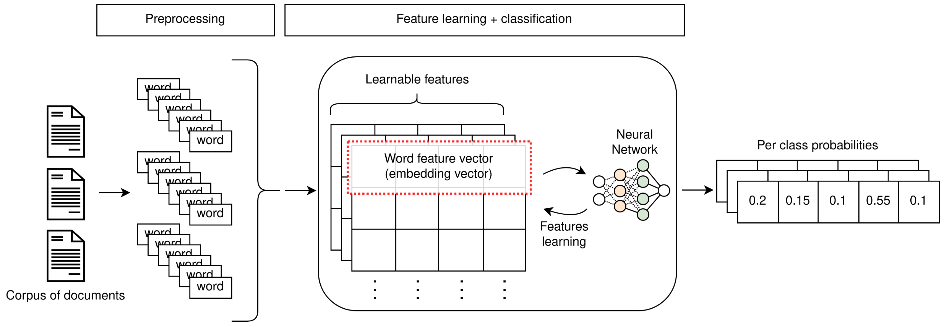
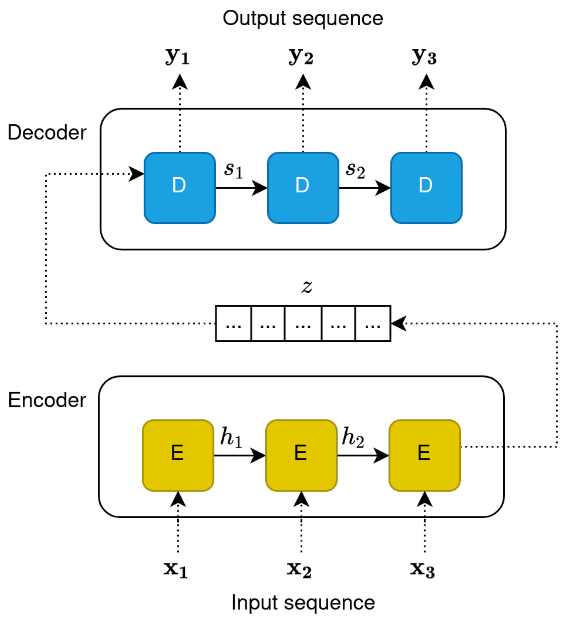
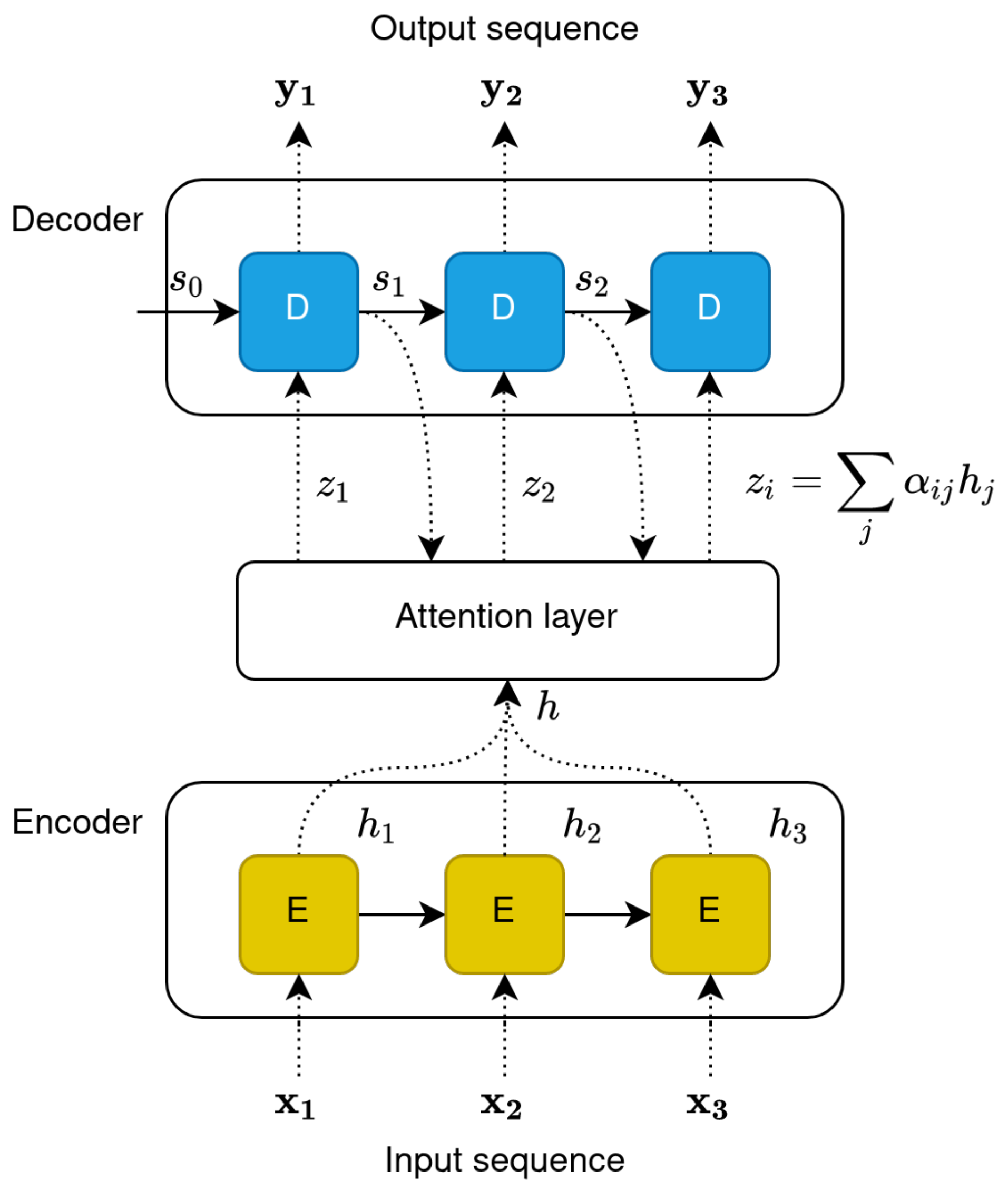
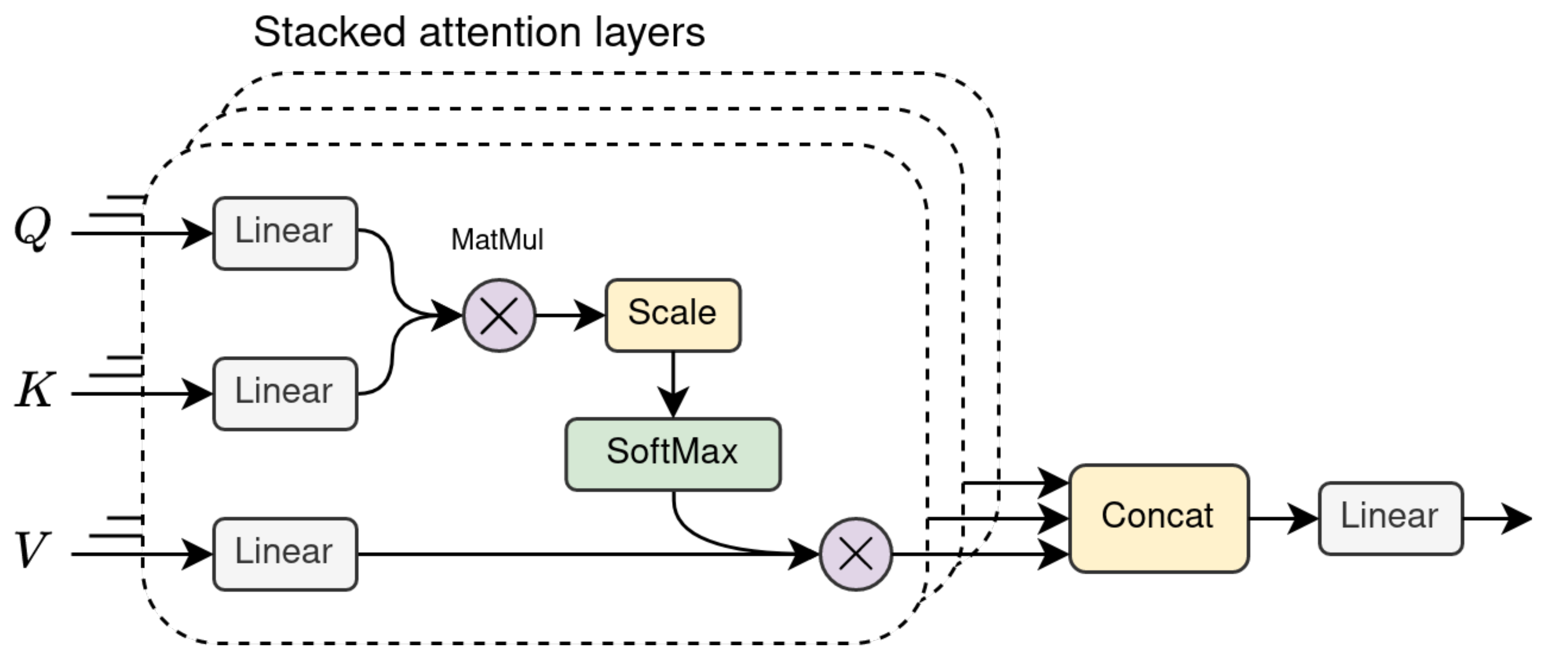
Table 3.
English TC datasets.
| Name | Task | Classes | Multilabel | Samples | |
|---|---|---|---|---|---|
| AG News [122] | NC | 4 | ✗ | 127,600 | |
| 20 News (20 Newsgroup) [123] | NC | 20 | ✗ | 18,846 | |
| R52 [124] | NC | 52 | ✗ | 9100 | |
| R8 [124] | NC | 8 | ✗ | 7674 | |
| Yelp2 (Yelp Polarity) [125,126] | SA | 2 | ✗ | 598,000 | |
| Yelp5 (Yelp Full) [125,126] | SA | 5 | ✗ | 700,000 | |
| Amz2 (Amazon Polarity) [125] | SA | 2 | ✗ | 4,000,000 | |
| Amz5 (Amazon Full) [125] | SA | 5 | ✗ | 3,650,000 | |
| IMDb [127] | SA | 2 | ✗ | 50,000 | |
| IMDb10 [127] | SA | 10 | ✗ | 50,000 | |
| MR (Movie Review) [128] | SA | 2 | ✗ | 10,662 | |
| Yah!A (Yahoo! Answers) [125] | TL | 10 | ✗ | 1,450,000 | |
| TREC [129] | TL | 6 | ✗ | 5952 | |
| Ohs (Ohsumed) [130,131] | TL | 23 | ✓ | 13,929 | |
| DBP (DBpedia-14) [125] | TL | 14 | ✗ | 630,000 | |
| EnWiki-100 1 | TL | 100 | ✓ | 329,600 | |
| RCV1-57 1 | NC | 57 | ✓ | 758,100 |
Datasets presented in this paper.
6.2. Evaluation Metrics
Accuracy is the most adopted evaluation metric for TC tasks. This metric is a simple and interpretable way of measuring the overall fraction of correct predictions. It is defined as the number of correct predictions over the total number of samples (N), as in Equation (6). The equations use standard notations for evaluation metrics, namely true positive (TP), true negative (TN), false positive (FP), and false negative (FN).
In a multilabel setting, the definition of this metric can change depending on the definition of true positives and negatives. A prediction may be considered correct when the predicted labels exactly match the ground truth (referred to as “subset accuracy”). Alternatively, predictions can be flattened and reduced to a single-label task before the accuracy computation.
Precision and recall are other popular metrics, especially for multilabel classification. The former is the fraction of correct predictions among all the ones that have been predicted as true (), while the latter is the fraction of correct predictions over all the ones that should have been predicted (). F-score, and in particular F1-score, is a popular combination of these two; it is defined as the harmonic mean of precision and recall, as in Equation (7).
For multilabel and multiclass problems, these metrics can be computed separately for each class and then averaged, obtaining the macro-averaged metrics. In such a case, every class contributes equally to the final score, and hence provides a more challenging metric for unbalanced datasets. On the other hand, a micro-average reduction strategy is used when computing the metric globally with no weighting.
6.3. Quantitative Results
The accuracy score for several previously introduced algorithms on prominent benchmarks are shown in Table 4 and Table 5. We report only accuracy, since it is the most consistently used metric across different studies. GLUE and RACE benchmarks are popular choices for the evaluation of NLP methods on a variety of tasks, hence we report results on these datasets in Table 6, whenever available. We evaluated a selection of deep and shallow methods on our new synthesised datasets. Since our datasets are multilabel, we report the F1-score with macro-averaging across all categories, along with the subset accuracy, computed on the test set. Table 4 and Table 5 showcases our results, averaged on four different evaluation splits. The following section provides additional details on the training procedure.
6.3.1. Custom Experimental Setup
We selected seven algorithms (Table 7) that either were recently, or have been, state-of-the-art approaches in TC tasks, and we test their performances on the EnWiki-100 and RCV1-57 datasets to showcase their performances on new multilabel datasets. As strong baseline representatives for classical methods, we present the results of Naïve Bayes and linear support vector classifiers, both using TF-IDF features. These methods are utilised in a one-vs.-rest ensemble fashion, as is common in multilabel applications. We then present the results of FastText [53], a re-implementation of XML-CNN [118,133] and a BiLSTM-based classifier as representatives of those methods bridging the gap between earlier methods and DLMs. Lastly, we fine-tuned and tested Transformer-based language models utilising the pre-trained open-source models, published in the Hugging Face library [158].
Datasets are split into training, validation, and test set: 40% of the data are reserved for testing, and 20% of the remaining samples are used for validation. Splits are produced in a way to preserve the distribution of labels, through a stratification strategy [159,160]. Final metrics reported in Table 7 are obtained by averaging results on the test set over all runs (four runs of each method, except for XLM-R, due to computational complexity). Hyperparameters for the Naïve Bayes and SVM classifiers are tuned using a grid search with 10 fold cross-validation. FastText hyperparameters are selected using the auto-tuning procedure provided in the Python package. Due to resource constraints, only a limited tuning of the most impactful parameters is performed on the bidirectional LSTM and Transformer-based models.
6.3.2. Discussion on Results
Table 4 and Table 5 show the dominance of Transformer-based language models in all TC tasks. Specifically, BERT and XLNet reach state-of-the-art performances on most datasets. Moreover, TC using graph representation for documents, paired with graph convolutional networks, proves to be an effective approach for the extraction of useful features, especially when node embeddings are initialized with contextual representations generated by BERT-like models (BertGCN, RoBERTaGCN). Notably, Thongtan and Phienthrakul [144] propose to learn document-level embeddings by minimising cosine similarity, and combining features extracted from a Naïve Bayes model before the classification step. The model architecture is very simple in comparison with BERT and other deeper language models, but manages to achieve the best accuracy on a binary SA dataset. The authors argue that, for this kind of task, tailored document representations are more important than the choice of classifier. Abreu et al. [71] achieve state-of-the-art results on the Yelp5 dataset, by using a CNN to extract features from word vectors and using the attention mechanism twice, first at the word level, to generate a sentence representation, and then at the sentence level, to weight the importance of sentences in the document embedding used for classification. This model makes use of recurrent blocks (GRU) and reiterates the importance of the attention mechanism to enhance seq2seq architectures.
The latest trend for the evaluation of deep language models is the leveraging of general multi-task benchmarks. Table 6 showcases the results of two of them. These benchmarks measure the model ability to generalise to multiple tasks, and are not specific for TC. The reported score averages the performance metrics of the model across all tasks.
Finally, Table 7 lists the results that we obtained on the new synthesised multilabel datasets. Since these are new datasets, we use them to test the classification performance of a few notable language models, within the limits of our resources. Unsurprisingly, BERT and XML-R achieved the best results over the two new corpora, with accuracy values aligned with the respective scores of similar multilabel TL datasets (e.g., Ohsumed). We clarify that, since these datasets are different, metrics should not be directly compared, but we expected classification accuracy to fall in a range of values that are reasonably comparable to the other TL datasets. Interestingly, XML-R performed only slightly worse than BERT, despite being a multilingual model which was not specifically trained to understand the English language. On the one side, this is interesting, as the curse of multilinguality—which states that the per-language capacity decreases as the number of languages grows—suggests that BERT should be able to understand much better the single language that it was trained on. On the other hand, one should consider that the smaller XML-R model has more than 2.5 times the parameters of the BERT base, and the two models are pre-trained on different corpora. XML-R is pre-trained on the Common Crawl in 100 languages, while our BERT model is pre-trained on the combination of BookCorpus and Wikipedia dumps. While the former corpus amounts to 2.5 TB of data, the latter does not exceed one hundred GB. The BiLSTM also performed better than other non-Transformer methods, as expected, since its architecture makes it suitable to model dependencies between adjacent chunks of text.
7. Future Research Directions
Despite achieving state-of-the-art results throughout NLP literature, large-scale language models are not infallible. For example, recent studies [161,162] reported that BERT models show considerable performance pitfalls when faced with adversarial text examples generated by adversarial networks. These text sequences are subtly altered with word-level replacements or sentence rephrasings that do not change their meaning (as far as human understanding is concerned), but are enough to fool these language models. This phenomenon raises questions about the ability of these models to make decisions based on the actual meaning carried by a portion of text. Particularly interesting is therefore the development of robustness benchmarks such as AdvGLUE [163], which aim to quantitatively and thoroughly explore the vulnerabilities of modern large-scale language models. Such benchmarks are carefully filtered and validated by human annotators, such as to ensure that adversarial examples are valid and unambiguous. Benchmarks like these will be fundamental in the development of more sophisticated adversarial attacks, as well as more robust language models able to withstand them.
The current trend of proposing deeper and deeper models with an ever-increasing number of parameters has led some scientists to warn against the creation of so-called “stochastic parrots” that effectively emulate language understanding by memorising large training datasets, but with very limited actual generalisation ability, let alone the ability to comprehend human language. Furthermore, the black-box nature of deep neural networks adds to these concerns, as learnt features are hardly interpretable, while some computational linguists also bring legitimate concern about harmful and dangerous biases learnt from the data [79]. As a consequence, future research should put the robustness of large-scale language models under mindful scrutiny and provide tools to lessen the interpretability issues which currently afflict deep learning. The former problem is addressed by Wang et al. [164], who propose a framework for a more robust fine-tuning of BERT language models.
Finally, recent developments have gone against the trend of scaling larger and larger models, proposing that smaller generative LMs can perform competitively with massively larger models when augmented with search/query information from a retrieval database [165,166]. For example, Retrieval-Enhanced Transformer (RETRO) performs on par with GPT-3, despite being 4% its size. Pursuing more reasonably sized models is certainly a research direction that will be worth exploring.
8. Conclusions
In this manuscript, we provide an overview of existing models for text classification (TC), highlighting the steps necessary to encode textual data into a feature space for classification. We presented an analysis of preprocessing operations for both shallow and deep learning methods, exploring procedures that are often taken for granted. We outlined the development in the approaches to NLP tasks and TC in particular, showcasing how they have evolved, up to the very recent Transformer-based methods. We provided an overview of English datasets, while also laying out instructions to synthesise two new multilabel classification datasets. We move towards the conclusion by presenting experimental results for methods as researched in the literature, as well as new results on our datasets for a choice of methods. Finally, we explore future research challenges, mainly tied to the robustness of DLMs and what is being done to address their weaknesses.
Author Contributions
Conceptualization, A.G., A.Z. and M.M.; methodology, A.Z.; software, A.Z. and M.M.; validation, A.G., A.Z. and M.M.; formal analysis, M.M.; investigation, A.Z. and M.M.; resources, A.Z.; data curation, A.Z.; writing—original draft preparation, A.Z. and M.M.; writing—review and editing, A.G., A.Z. and M.M.; visualization, A.Z. and M.M.; supervision, A.G. and A.A.; project administration, A.G. and A.A. All authors have read and agreed to the published version of the manuscript.
Funding
This research received no external funding.
Institutional Review Board Statement
Not applicable.
Informed Consent Statement
Not applicable.
Data Availability Statement
Publicly available datasets were analysed in this study. These data, along with all the code produced, can be found here: https://gitlab.com/distration/dsi-nlp-publib (accessed on 28 December 2021).
Acknowledgments
We would like to thank NIST for allowing us to utilise the RCV1 dataset in our experiments.
Conflicts of Interest
The authors declare no conflict of interest.
Abbreviations
The following abbreviations are used in this manuscript:
| TC | Text Classification |
| NLP | Natural Language Processing |
| DLM | Deep Language Model |
| CNN | Convolutional Neural Network |
| RNN | Recurrent Neural Network |
| LSTM | Long Short-Term Memory (Network) |
| GRU | Gated Recurrent Units |
| OOV | Out-of-Vocabulary (word) |
| BERT | Bidirectional Encoder Representations from Transformers |
| GPT | Generative Pre-trained Transformer |
| GNN | Graph Neural Network |
| MHA | Multi-Head Attention |
References
- Li, Q.; Peng, H.; Li, J.; Xia, C.; Yang, R.; Sun, L.; Yu, P.S.; He, L. A Survey on Text Classification: From Shallow to Deep Learning. arXiv 2020, arXiv:2008.00364. [Google Scholar]
- Kowsari, K.; Jafari Meimandi, K.; Heidarysafa, M.; Mendu, S.; Barnes, L.; Brown, D. Text Classification Algorithms: A Survey. Information 2019, 10, 150. [Google Scholar] [CrossRef] [Green Version]
- Minaee, S.; Kalchbrenner, N.; Cambria, E.; Nikzad, N.; Chenaghlu, M.; Gao, J. Deep Learning–Based Text Classification: A Comprehensive Review. Acm Comput. Surv. 2021, 54, 1–40. [Google Scholar] [CrossRef]
- Graves, A. Generating Sequences With Recurrent Neural Networks. arXiv 2013, arXiv:1308.0850. [Google Scholar]
- Manning, C.D.; Raghavan, P.; Schütze, H. Introduction to Information Retrieval; Cambridge University Press: Cambridge, UK, 2008. [Google Scholar] [CrossRef]
- Mielke, S.J.; Alyafeai, Z.; Salesky, E.; Raffel, C.; Dey, M.; Gallé, M.; Raja, A.; Si, C.; Lee, W.Y.; Sagot, B.; et al. Between words and characters: A Brief History of Open-Vocabulary Modeling and Tokenization in NLP. arXiv 2021, arXiv:2112.10508. [Google Scholar]
- Saif, H.; Fernandez, M.; He, Y.; Alani, H. On Stopwords, Filtering and Data Sparsity for Sentiment Analysis of Twitter. In Proceedings of the Ninth International Conference on Language Resources and Evaluation (LREC’14), Reykjavik, Iceland, 26–31 May 2014; pp. 810–817. [Google Scholar]
- Jivani, A. A Comparative Study of Stemming Algorithms. Int. J. Comput. Technol. Appl. 2011, 2, 1930–1938. [Google Scholar]
- Plisson, J.; Lavrac, N.; Mladenic, D. A rule based approach to word lemmatization. In Proceedings of the 7th International Multiconference on Information Society (IS04), Ljubljana, Slovenia, 11–15 October 2004. [Google Scholar]
- Gage, P. A New Algorithm for Data Compression. C Users J. 1994, 12, 23–38. [Google Scholar]
- Sennrich, R.; Haddow, B.; Birch, A. Neural Machine Translation of Rare Words with Subword Units. In Proceedings of the 54th Annual Meeting of the Association for Computational Linguistics, Berlin, Germany, 7–12 August 2016; pp. 1715–1725. [Google Scholar] [CrossRef]
- Radford, A.; Wu, J.; Child, R.; Luan, D.; Amodei, D.; Sutskever, I. Language Models are Unsupervised Multitask Learners. OpenAI Blog 2019, 1, 9. [Google Scholar]
- Liu, Y.; Ott, M.; Goyal, N.; Du, J.; Joshi, M.; Chen, D.; Levy, O.; Lewis, M.; Zettlemoyer, L.; Stoyanov, V. RoBERTa: A Robustly Optimized BERT Pretraining Approach. arXiv 2019, arXiv:1907.11692. [Google Scholar]
- Wang, C.; Cho, K.; Gu, J. Neural Machine Translation with Byte-Level Subwords. Proc. AAAI Conf. Artif. Intell. 2020, 34, 9154–9160. [Google Scholar] [CrossRef]
- Schuster, M.; Nakajima, K. Japanese and Korean voice search. In Proceedings of the 2012 IEEE International Conference on Acoustics, Speech and Signal Processing (ICASSP), Kyoto, Japan, 25–30 March 2012; pp. 5149–5152. [Google Scholar]
- Devlin, J.; Chang, M.W.; Lee, K.; Toutanova, K. BERT: Pre-training of Deep Bidirectional Transformers for Language Understanding. In Proceedings of the 2019 Conference of the North American Chapter of the Association for Computational Linguistics: Human Language Technologies, Minnesota, MN, USA, 2–7 June 2019; pp. 4171–4186. [Google Scholar]
- Kudo, T. Subword Regularization: Improving Neural Network Translation Models with Multiple Subword Candidates. In Proceedings of the 56th Annual Meeting of the Association for Computational Linguistics (Volume 1: Long Papers), Melbourne, Australia, 15–20 July 2018; pp. 66–75. [Google Scholar] [CrossRef] [Green Version]
- Kudo, T.; Richardson, J. SentencePiece: A simple and language independent subword tokenizer and detokenizer for Neural Text Processing. In Proceedings of the 2018 Conference on Empirical Methods in Natural Language Processing: System Demonstrations, Brussels, Belgium, 31 October–4 November 2018; pp. 66–71. [Google Scholar] [CrossRef] [Green Version]
- Yang, Z.; Dai, Z.; Yang, Y.; Carbonell, J.; Salakhutdinov, R.; Le, Q.V. XLNet: Generalized Autoregressive Pretraining for Language Understanding. In Proceedings of the 33rd International Conference on Neural Information Processing Systems, Vancouver, BC, Canada, 8–14 December 2019. [Google Scholar]
- Conneau, A.; Khandelwal, K.; Goyal, N.; Chaudhary, V.; Wenzek, G.; Guzmán, F.; Grave, E.; Ott, M.; Zettlemoyer, L.; Stoyanov, V. Unsupervised Cross-lingual Representation Learning at Scale. In Proceedings of the 58th Annual Meeting of the Association for Computational Linguistics, Online event, 5–10 July 2020; pp. 8440–8451. [Google Scholar] [CrossRef]
- Rodolà, E.; Cosmo, L.; Litany, O.; Bronstein, M.M.; Bronstein, A.M.; Audebert, N.; Hamza, A.B.; Boulch, A.; Castellani, U.; Do, M.N.; et al. Deformable Shape Retrieval with Missing Parts. In Proceedings of the Eurographics Workshop on 3D Object Retrieval, Lyon, France, 23–24 April 2017; Pratikakis, I., Dupont, F., Ovsjanikov, M., Eds.; Eurographics Association: Geneva, Switzerland, 2017. [Google Scholar] [CrossRef]
- Gasparetto, A.; Minello, G.; Torsello, A. Non-parametric Spectral Model for Shape Retrieval. In Proceedings of the 2015 International Conference on 3D Vision, Lyon, France, 19–22 October 2015; pp. 344–352. [Google Scholar] [CrossRef]
- Pistellato, M.; Bergamasco, F.; Albarelli, A.; Cosmo, L.; Gasparetto, A.; Torsello, A. Robust phase unwrapping by probabilistic consensus. Opt. Lasers Eng. 2019, 121, 428–440. [Google Scholar] [CrossRef]
- Jones, K.S. A statistical interpretation of term specificity and its application in retrieval. J. Doc. 1972, 28, 11–21. [Google Scholar] [CrossRef]
- Maćkiewicz, A.; Ratajczak, W. Principal components analysis (PCA). Comput. Geosci. 1993, 19, 303–342. [Google Scholar] [CrossRef]
- Tharwat, A.; Gaber, T.; Ibrahim, A.; Hassanien, A.E. Linear discriminant analysis: A detailed tutorial. Ai Commun. 2017, 30, 169–190. [Google Scholar] [CrossRef] [Green Version]
- Tsuge, S.; Shishibori, M.; Kuroiwa, S.; Kita, K. Dimensionality reduction using non-negative matrix factorization for information retrieval. In Proceedings of the 2001 IEEE International Conference on Systems, Man and Cybernetics. e-Systems and e-Man for Cybernetics in Cyberspace (Cat.No.01CH37236), Tucson, AZ, USA, 7–10 October 2001; Volume 2, pp. 960–965. [Google Scholar] [CrossRef]
- Rosenfeld, R. Two decades of statistical language modeling: Where do we go from here? Proc. IEEE 2000, 88, 1270–1278. [Google Scholar] [CrossRef]
- Jurafsky, D.; Martin, J. Speech and Language Processing: An Introduction to Natural Language Processing, Computational Linguistics, and Speech Recognition, 3rd ed. (draft) Unpublished. 2021, pp. 30–35. Available online: https://web.stanford.edu/~jurafsky/slp3/ed3book.pdf (accessed on 28 December 2021).
- Huang, E.H.; Socher, R.; Manning, C.D.; Ng, A.Y. Improving Word Representations via Global Context and Multiple Word Prototypes. In Proceedings of the 50th Annual Meeting of the Association for Computational Linguistics, Jeju Island, Korea, 8–14 July 2012; Volume 1, pp. 873–882. [Google Scholar]
- Mikolov, T.; Chen, K.; Corrado, G.; Dean, J. Efficient Estimation of Word Representations in Vector Space. In Proceedings of the 1st International Conference on Learning Representations (ICLR 2013), Scottsdale, AZ, USA, 2–4 May 2013. [Google Scholar]
- Mikolov, T.; Sutskever, I.; Chen, K.; Corrado, G.S.; Dean, J. Distributed Representations of Words and Phrases and their Compositionality. In Proceedings of the 26th International Conference on Neural Information Processing Systems, Lake Tahoe, NV, USA, 5–10 December 2013; Volume 2, pp. 3111–3119. [Google Scholar]
- Pennington, J.; Socher, R.; Manning, C. GloVe: Global Vectors for Word Representation. In Proceedings of the 2014 Conference on Empirical Methods in Natural Language Processing (EMNLP), Doha, Qatar, 25–29 October 2014; pp. 1532–1543. [Google Scholar] [CrossRef]
- Baroni, M.; Dinu, G.; Kruszewski, G. Don’t count, predict! A systematic comparison of context-counting vs. context-predicting semantic vectors. In Proceedings of the 52nd Annual Meeting of the Association for Computational Linguistics, Baltimore, MD, USA, 22–27 June 2014; Volume 1, pp. 238–247. [Google Scholar] [CrossRef] [Green Version]
- Bojanowski, P.; Grave, E.; Joulin, A.; Mikolov, T. Enriching Word Vectors with Subword Information. Trans. Assoc. Comput. Linguist. 2017, 5, 135–146. [Google Scholar] [CrossRef] [Green Version]
- Xu, S.; Li, Y.; Wang, Z. Bayesian Multinomial Naïve Bayes Classifier to Text Classification. In Advanced Multimedia and Ubiquitous Engineering; Springer: Singapore, 2017; pp. 347–352. [Google Scholar] [CrossRef]
- Van den Bosch, A. Hidden Markov Models. In Encyclopedia of Machine Learning and Data Mining; Springer: Boston, MA, USA, 2017; pp. 609–611. [Google Scholar] [CrossRef]
- Sutton, C.; McCallum, A. An Introduction to Conditional Random Fields. Found. Trends® Mach. Learn. 2012, 4, 267–373. [Google Scholar] [CrossRef]
- Cover, T.; Hart, P. Nearest Neighbor pattern classification. IEEE Trans. Inf. Theory 1967, 13, 21–27. [Google Scholar] [CrossRef]
- Li, B.; Yu, S.; Lu, Q. An Improved k-Nearest Neighbor Algorithm for Text Categorization. arXiv 2003, arXiv:cs/0306099. [Google Scholar]
- Ali, N.; Neagu, D.; Trundle, P. Evaluation of k-nearest neighbour classifier performance for heterogeneous data sets. SN Appl. Sci. 2019, 1, 1–15. [Google Scholar] [CrossRef] [Green Version]
- Bellman, R. Dynamic Programming. Science 1966, 153, 34–37. [Google Scholar] [CrossRef] [PubMed]
- Cortes, C.; Vapnik, V.N. Support-Vector Networks. Mach. Learn. 1995, 20, 273–297. [Google Scholar] [CrossRef]
- Boser, B.E.; Guyon, I.M.; Vapnik, V.N. A Training Algorithm for Optimal Margin Classifiers. In Proceedings of the Fifth Annual Workshop on Computational Learning Theory, Pittsburgh, PA, USA, 27–29 July 1992; pp. 144–152. [Google Scholar] [CrossRef]
- Safavian, S.; Landgrebe, D. A survey of decision tree classifier methodology. IEEE Trans. Syst. Man Cybern. 1991, 21, 660–674. [Google Scholar] [CrossRef] [Green Version]
- Ho, T.K. Random decision forests. In Proceedings of the 3rd International Conference on Document Analysis and Recognition, Montreal, QC, Canada, 14–15 August 1995; Volume 1, pp. 278–282. [Google Scholar] [CrossRef]
- Islam, M.Z.; Liu, J.; Li, J.; Liu, L.; Kang, W. A Semantics Aware Random Forest for Text Classification. In Proceedings of the 28th ACM International Conference on Information and Knowledge Management (CIKM ’19), Beijing, China, 3–7 November 2019; pp. 1061–1070. [Google Scholar] [CrossRef] [Green Version]
- Genkin, A.; Lewis, D.; Madigan, D. Large-Scale Bayesian Logistic Regression for Text Categorization. Technometrics 2007, 49, 291–304. [Google Scholar] [CrossRef] [Green Version]
- Krishnapuram, B.; Carin, L.; Figueiredo, M.; Hartemink, A. Sparse multinomial logistic regression: Fast algorithms and generalization bounds. IEEE Trans. Pattern Anal. Mach. Intell. 2005, 27, 957–968. [Google Scholar] [CrossRef] [Green Version]
- Breiman, L. Bagging predictors. Mach. Learn. 2004, 24, 123–140. [Google Scholar] [CrossRef] [Green Version]
- Schapire, R.E. The Strength of Weak Learnability. Mach. Learn. 1990, 5, 197–227. [Google Scholar] [CrossRef] [Green Version]
- Freund, Y.; Schapire, R.E. A Decision-Theoretic Generalization of On-Line Learning and an Application to Boosting. J. Comput. Syst. Sci. 1997, 55, 119–139. [Google Scholar] [CrossRef] [Green Version]
- Joulin, A.; Grave, E.; Bojanowski, P.; Mikolov, T. Bag of Tricks for Efficient Text Classification. In Proceedings of the 15th Conference of the European Chapter of the Association for Computational Linguistics, Valencia, Spain, 3–7 April 2017; Volume 2, pp. 427–431. [Google Scholar]
- Ibrahim, M.A.; Ghani Khan, M.U.; Mehmood, F.; Asim, M.N.; Mahmood, W. GHS-NET a generic hybridized shallow neural network for multi-label biomedical text classification. J. Biomed. Inform. 2021, 116, 103699. [Google Scholar] [CrossRef]
- Iyyer, M.; Manjunatha, V.; Boyd-Graber, J.; Daumé, H., III. Deep Unordered Composition Rivals Syntactic Methods for Text Classification. In Proceedings of the 53rd Annual Meeting of the Association for Computational Linguistics and the 7th International Joint Conference on Natural Language Processing, Beijing, China, 27–31 July 2015; Volume 1, pp. 1681–1691. [Google Scholar] [CrossRef]
- Le, Q.; Mikolov, T. Distributed Representations of Sentences and Documents. In Proceedings of the 31st International Conference on Machine Learning, Beijing, China, 21–26 June 2014; Volume 32, pp. 1188–1196. [Google Scholar]
- Mikolov, T.; Le, Q.V.; Sutskever, I. Exploiting Similarities among Languages for Machine Translation. arXiv 2013, arXiv:1309.4168. [Google Scholar]
- Hochreiter, S.; Schmidhuber, J. Long Short-term Memory. Neural Comput. 1997, 9, 1735–1780. [Google Scholar] [CrossRef] [PubMed]
- Tai, K.S.; Socher, R.; Manning, C.D. Improved Semantic Representations From Tree-Structured Long Short-Term Memory Networks. In Proceedings of the 53rd Annual Meeting of the Association for Computational Linguistics and the 7th International Joint Conference on Natural Language Processing, Beijing, China, 27–31 July 2015; Volume 1, pp. 1556–1566. [Google Scholar] [CrossRef] [Green Version]
- Dieng, A.B.; Wang, C.; Gao, J.; Paisley, J. TopicRNN: A Recurrent Neural Network with Long-Range Semantic Dependency. arXiv 2016, arXiv:1611.01702. [Google Scholar]
- Howard, J.; Ruder, S. Universal Language Model Fine-tuning for Text Classification. In Proceedings of the 56th Annual Meeting of the Association for Computational Linguistics, Melbourne, Australia, 15–20 July 2018; Volume 1, pp. 328–339. [Google Scholar] [CrossRef] [Green Version]
- Wang, B. Disconnected Recurrent Neural Networks for Text Categorization. In Proceedings of the 56th Annual Meeting of the Association for Computational Linguistics, Melbourne, Australia, 15–20 July 2018; Volume 1, pp. 2311–2320. [Google Scholar] [CrossRef] [Green Version]
- Cho, K.; van Merriënboer, B.; Gulcehre, C.; Bahdanau, D.; Bougares, F.; Schwenk, H.; Bengio, Y. Learning Phrase Representations using RNN Encoder–Decoder for Statistical Machine Translation. In Proceedings of the 2014 Conference on Empirical Methods in Natural Language Processing (EMNLP), Doha, Qatar, 25–29 October 2014; pp. 1724–1734. [Google Scholar] [CrossRef]
- Schuster, M.; Paliwal, K. Bidirectional recurrent neural networks. IEEE Trans. Signal Process. 1997, 45, 2673–2681. [Google Scholar] [CrossRef] [Green Version]
- Peters, M.E.; Neumann, M.; Iyyer, M.; Gardner, M.; Clark, C.; Lee, K.; Zettlemoyer, L. Deep Contextualized Word Representations. In Proceedings of the 2018 Conference of the North American Chapter of the Association for Computational Linguistics: Human Language Technologies, New Orleans, LA, USA, 1–6 June 2018; Volume 1, pp. 2227–2237. [Google Scholar] [CrossRef] [Green Version]
- Zhang, Y.; Wallace, B.C. A Sensitivity Analysis of (and Practitioners’ Guide to) Convolutional Neural Networks for Sentence Classification. In Proceedings of the Eighth International Joint Conference on Natural Language Processing (IJCNLP), Taipei, Taiwan, 27–30 November 2017; Volume 1, pp. 253–263. [Google Scholar]
- Stone, A.; Wang, H.; Stark, M.; Liu, Y.; Phoenix, D.; George, D. Teaching Compositionality to CNNs. In Proceedings of the 2017 IEEE Conference on Computer Vision and Pattern Recognition (CVPR), Honolulu, HI, USA, 21–26 July 2017; pp. 732–741. [Google Scholar] [CrossRef] [Green Version]
- Pistellato, M.; Cosmo, L.; Bergamasco, F.; Gasparetto, A.; Albarelli, A. Adaptive Albedo Compensation for Accurate Phase-Shift Coding. In Proceedings of the 2018 24th International Conference on Pattern Recognition (ICPR), Beijing, China, 20–24 August 2018; pp. 2450–2455. [Google Scholar] [CrossRef]
- Kim, Y. Convolutional Neural Networks for Sentence Classification. In Proceedings of the 2014 Conference on Empirical Methods in Natural Language Processing (EMNLP), Doha, Qatar, 25–29 October 2014; pp. 1746–1751. [Google Scholar] [CrossRef] [Green Version]
- Lea, C.; Flynn, M.D.; Vidal, R.; Reiter, A.; Hager, G.D. Temporal Convolutional Networks for Action Segmentation and Detection. In Proceedings of the 2017 IEEE Conference on Computer Vision and Pattern Recognition (CVPR), Honolulu, HI, USA, 21–26 July 2017; pp. 1003–1012. [Google Scholar] [CrossRef] [Green Version]
- Abreu, J.; Fred, L.; Macêdo, D.; Zanchettin, C. Hierarchical Attentional Hybrid Neural Networks for Document Classification. In Artificial Neural Networks and Machine Learning—ICANN 2019: Workshop and Special Sessions; Springer International Publishing: Cham, Switzerland, 2019; pp. 396–402. [Google Scholar] [CrossRef] [Green Version]
- Yan, J.; Mu, L.; Wang, L.; Ranjan, R.; Zomaya, A.Y. Temporal Convolutional Networks for the Advance Prediction of ENSO. Sci. Rep. 2020, 10, 8055. [Google Scholar] [CrossRef]
- Conneau, A.; Schwenk, H.; Barrault, L.; Lecun, Y. Very Deep Convolutional Networks for Text Classification. In Proceedings of the 15th Conference of the European Chapter of the Association for Computational Linguistics, Valencia, Spain, 3–7 April 2017; Volume 1, pp. 1107–1116. [Google Scholar]
- Duque, A.B.; Santos, L.L.J.; Macêdo, D.; Zanchettin, C. Squeezed Very Deep Convolutional Neural Networks for Text Classification. In Artificial Neural Networks and Machine Learning—ICANN 2019: Theoretical Neural Computation; Springer International Publishing: Cham, Switzerland, 2019; pp. 193–207. [Google Scholar] [CrossRef] [Green Version]
- Sutskever, I.; Vinyals, O.; Le, Q.V. Sequence to Sequence Learning with Neural Networks. In Proceedings of the 27th International Conference on Neural Information Processing Systems, Montreal, QC, Canada, 8–13 December 2014; MIT Press: Cambridge, MA, USA, 2014; Volume 2, pp. 3104–3112. [Google Scholar]
- Bahdanau, D.; Cho, K.; Bengio, Y. Neural Machine Translation by Jointly Learning to Align and Translate. arXiv 2015, arXiv:1409.0473. [Google Scholar]
- Pascanu, R.; Mikolov, T.; Bengio, Y. On the difficulty of training recurrent neural networks. In Proceedings of the 30th International Conference on Machine Learning, Atlanta, GA, USA, 16–21 June 2013; Dasgupta, S., McAllester, D., Eds.; PMLR: Atlanta, GA, USA, 2013; Volume 28, pp. 1310–1318. [Google Scholar]
- Luong, T.; Pham, H.; Manning, C.D. Effective Approaches to Attention-based Neural Machine Translation. In Proceedings of the 2015 Conference on Empirical Methods in Natural Language Processing, Lisbon, Portugal, 17–21 September 2015; pp. 1412–1421. [Google Scholar] [CrossRef] [Green Version]
- Bender, E.M.; Gebru, T.; McMillan-Major, A.; Shmitchell, S. On the Dangers of Stochastic Parrots: Can Language Models Be Too Big? In Proceedings of the 2021 ACM Conference on Fairness, Accountability, and Transparency, Online event, 3–10 March 2021; pp. 610–623. [Google Scholar] [CrossRef]
- Yang, Z.; Yang, D.; Dyer, C.; He, X.; Smola, A.; Hovy, E. Hierarchical Attention Networks for Document Classification. In Proceedings of the 2016 Conference of the North American Chapter of the Association for Computational Linguistics: Human Language Technologies, San Diego, CA, USA, 12–17 June 2016; pp. 1480–1489. [Google Scholar] [CrossRef] [Green Version]
- Vaswani, A.; Shazeer, N.; Parmar, N.; Uszkoreit, J.; Jones, L.; Gomez, A.N.; Kaiser, L.; Polosukhin, I. Attention is All You Need. In Proceedings of the 31st International Conference on Neural Information Processing Systems, Long Beach, CA, USA, 4–9 December 2017; pp. 6000–6010. [Google Scholar]
- Liu, P.J.; Saleh, M.; Pot, E.; Goodrich, B.; Sepassi, R.; Kaiser, L.; Shazeer, N. Generating Wikipedia by Summarizing Long Sequences. arXiv 2018, arXiv:1801.10198. [Google Scholar]
- Radford, A.; Narasimhan, K. Improving Language Understanding by Generative Pre-Training. OpenAI Blog. 2018. Available online: https://www.cs.ubc.ca/~amuham01/LING530/papers/radford2018improving.pdf (accessed on 28 December 2021).
- Von Platen, P. Transformers-Based Encoder-Decoder Models. Available online: https://huggingface.co/blog/encoder-decoder (accessed on 28 December 2021).
- Wang, A.; Singh, A.; Michael, J.; Hill, F.; Levy, O.; Bowman, S. GLUE: A Multi-Task Benchmark and Analysis Platform for Natural Language Understanding. In Proceedings of the 2018 EMNLP Workshop BlackboxNLP: Analyzing and Interpreting Neural Networks for NLP, Brussels, Belgium, 31 October–4 November 2018; pp. 353–355. [Google Scholar] [CrossRef] [Green Version]
- Brown, T.; Mann, B.; Ryder, N.; Subbiah, M.; Kaplan, J.D.; Dhariwal, P.; Neelakantan, A.; Shyam, P.; Sastry, G.; Askell, A.; et al. Language Models are Few-Shot Learners. In Proceedings of the 34th Annual Conference on Neural Information Processing Systems, Online event, 6–12 December 2020; Volume 33, pp. 1877–1901. [Google Scholar]
- Raffel, C.; Shazeer, N.; Roberts, A.; Lee, K.; Narang, S.; Matena, M.; Zhou, Y.; Li, W.; Liu, P.J. Exploring the Limits of Transfer Learning with a Unified Text-to-Text Transformer. J. Mach. Learn. Res. 2020, 21, 1–67. [Google Scholar]
- Sanh, V.; Webson, A.; Raffel, C.; Bach, S.H.; Sutawika, L.; Alyafeai, Z.; Chaffin, A.; Stiegler, A.; Scao, T.L.; Raja, A.; et al. Multitask Prompted Training Enables Zero-Shot Task Generalization. arXiv 2021, arXiv:2110.08207. [Google Scholar]
- He, P.; Liu, X.; Gao, J.; Chen, W. DeBERTa: Decoding-Enhanced BERT with Disentangled Attention. In Proceedings of the 2021 International Conference on Learning Representations (ICLR 2021), Vienna, Austria, 4–8 May 2021. [Google Scholar]
- Sun, Y.; Wang, S.; Feng, S.; Ding, S.; Pang, C.; Shang, J.; Liu, J.; Chen, X.; Zhao, Y.; Lu, Y.; et al. ERNIE 3.0: Large-scale Knowledge Enhanced Pre-training for Language Understanding and Generation. arXiv 2021, arXiv:2107.02137. [Google Scholar]
- Dai, Z.; Yang, Z.; Yang, Y.; Carbonell, J.; Le, Q.; Salakhutdinov, R. Transformer-XL: Attentive Language Models beyond a Fixed-Length Context. In Proceedings of the 57th Annual Meeting of the Association for Computational Linguistics, Florence, Italy, 28 July–2 August 2019; pp. 2978–2988. [Google Scholar] [CrossRef] [Green Version]
- Wei, J.; Bosma, M.; Zhao, V.Y.; Guu, K.; Yu, A.W.; Lester, B.; Du, N.; Dai, A.M.; Le, Q.V. Finetuned Language Models Are Zero-Shot Learners. arXiv 2021, arXiv:2109.01652. [Google Scholar]
- Schiavinato, M.; Gasparetto, A.; Torsello, A. Transitive assignment kernels for structural classification. Lect. Notes Comput. Sci. 2015, 9370, 146–159. [Google Scholar] [CrossRef]
- Cai, H.; Zheng, V.W.; Chang, K. A Comprehensive Survey of Graph Embedding: Problems, Techniques, and Applications. IEEE Trans. Knowl. Data Eng. 2018, 30, 1616–1637. [Google Scholar] [CrossRef] [Green Version]
- Battaglia, P.W.; Hamrick, J.B.; Bapst, V.; Sanchez-Gonzalez, A.; Zambaldi, V.F.; Malinowski, M.; Tacchetti, A.; Raposo, D.; Santoro, A.; Faulkner, R.; et al. Relational inductive biases, deep learning, and graph networks. arXiv 2018, arXiv:1806.01261. [Google Scholar]
- Bruna, J.; Zaremba, W.; Szlam, A.; Lecun, Y. Spectral networks and locally connected networks on graphs. In Proceedings of the International Conference on Learning Representations (ICLR 2014), Banff, AB, Canada, 14–16 April 2014. [Google Scholar]
- Torsello, A.; Gasparetto, A.; Rossi, L.; Bai, L.; Hancock, E. Transitive State Alignment for the Quantum Jensen-Shannon Kernel. Lect. Notes Comput. Sci. 2014, 8621, 22–31. [Google Scholar] [CrossRef] [Green Version]
- Yao, L.; Mao, C.; Luo, Y. Graph Convolutional Networks for Text Classification. Proc. AAAI Conf. Artif. Intell. 2019, 33, 7370–7377. [Google Scholar] [CrossRef] [Green Version]
- Church, K.W.; Hanks, P. Word Association Norms, Mutual Information, and Lexicography. In Proceedings of the 27th Annual Meeting on Association for Computational Linguistics, Vancouver, BC, Canada, 26–29 June 1989; pp. 76–83. [Google Scholar] [CrossRef]
- Lin, Y.; Meng, Y.; Sun, X.; Han, Q.; Kuang, K.; Li, J.; Wu, F. BertGCN: Transductive Text Classification by Combining GNN and BERT. In Findings of the Association for Computational Linguistics: ACL-IJCNLP 2021; Association for Computational Linguistics: Stroudsburg, PA, USA, 2021; pp. 1456–1462. [Google Scholar] [CrossRef]
- Nikolentzos, G.; Tixier, A.; Vazirgiannis, M. Message Passing Attention Networks for Document Understanding. Proc. AAAI Conf. Artif. Intell. 2020, 34, 8544–8551. [Google Scholar] [CrossRef]
- Gammerman, A.; Vovk, V.; Vapnik, V. Learning by Transduction. In Proceedings of the Fourteenth Conference on Uncertainty in Artificial Intelligence, Madison, WI, USA, 24–26 July 1998; pp. 148–155. [Google Scholar]
- Huang, L.; Ma, D.; Li, S.; Zhang, X.; Wang, H. Text Level Graph Neural Network for Text Classification. In Proceedings of the 2019 Conference on Empirical Methods in Natural Language Processing and the 9th International Joint Conference on Natural Language Processing (EMNLP-IJCNLP), Hong Kong, China, 3–7 November 2019; pp. 3444–3450. [Google Scholar] [CrossRef] [Green Version]
- Wu, F.; Souza, A.; Zhang, T.; Fifty, C.; Yu, T.; Weinberger, K. Simplifying Graph Convolutional Networks. In Proceedings of the 36th International Conference on Machine Learning, Irvine, CA, USA, 13–16 November 2019; Volume 9, pp. 6861–6871. [Google Scholar]
- Li, Q.; Han, Z.; Wu, X.M. Deeper Insights into Graph Convolutional Networks for Semi-Supervised Learning. In Proceedings of the Thirty-Second AAAI Conference on Artificial Intelligence, New Orleans, LA, USA, 2–7 February 2018. [Google Scholar]
- Chen, M.; Wei, Z.; Huang, Z.; Ding, B.; Li, Y. Simple and Deep Graph Convolutional Networks. In Proceedings of the 37th International Conference on Machine Learning, Online event, 13–18 July 2020; Volume 119, pp. 1725–1735. [Google Scholar]
- Zhu, H.; Koniusz, P. Simple Spectral Graph Convolution. In Proceedings of the 2021 International Conference on Learning Representations (ICLR 2021), Vienna, Austria, 4–8 May 2021. [Google Scholar]
- Klicpera, J.; Bojchevski, A.; Günnemann, S. Predict then Propagate: Graph Neural Networks meet Personalized PageRank. arXiv 2019, arXiv:1810.05997. [Google Scholar]
- Gasparetto, A.; Cosmo, L.; Rodola, E.; Bronstein, M.; Torsello, A. Spatial Maps: From low rank spectral to sparse spatial functional representations. In Proceedings of the 2017 International Conference on 3D Vision (3DV), Qingdao, China, 10–12 October 2017; pp. 477–485. [Google Scholar] [CrossRef]
- Ethayarajh, K. How Contextual are Contextualized Word Representations? Comparing the Geometry of BERT, ELMo, and GPT-2 Embeddings. In Proceedings of the 2019 Conference on Empirical Methods in Natural Language Processing and the 9th International Joint Conference on Natural Language Processing (EMNLP-IJCNLP), Hong Kong, China, 3–7 November 2019; pp. 55–65. [Google Scholar] [CrossRef]
- Peters, M.E.; Ammar, W.; Bhagavatula, C.; Power, R. Semi-supervised sequence tagging with bidirectional language models. In Proceedings of the 55th Annual Meeting of the Association for Computational Linguistics, Vancouver, BC, Canada, 31 July–4 August 2017; Volume 1, pp. 1756–1765. [Google Scholar] [CrossRef]
- McCann, B.; Bradbury, J.; Xiong, C.; Socher, R. Learned in Translation: Contextualized Word Vectors. In Proceedings of the 31st International Conference on Neural Information Processing Systems, Long Beach, CA, USA, 4–9 December 2017; Curran Associates Inc.: Red Hook, NY, USA, 2017; pp. 6297–6308. [Google Scholar]
- Hinton, G.; Vinyals, O.; Dean, J. Distilling the Knowledge in a Neural Network. arXiv 2015, arXiv:1503.02531. [Google Scholar]
- Sanh, V.; Debut, L.; Chaumond, J.; Wolf, T. DistilBERT, a distilled version of BERT: Smaller, faster, cheaper and lighter. arXiv 2019, arXiv:1910.01108. [Google Scholar]
- Jiao, X.; Yin, Y.; Shang, L.; Jiang, X.; Chen, X.; Li, L.; Wang, F.; Liu, Q. TinyBERT: Distilling BERT for Natural Language Understanding. In Proceedings of the Findings of the Association for Computational Linguistics: EMNLP 2020, Online event, 16–20 November 2020; pp. 4163–4174. [Google Scholar] [CrossRef]
- Lan, Z.; Chen, M.; Goodman, S.; Gimpel, K.; Sharma, P.; Soricut, R. ALBERT: A Lite BERT for Self-supervised Learning of Language Representations. arXiv 2019, arXiv:1909.11942. [Google Scholar]
- Clark, K.; Luong, M.T.; Le, Q.V.; Manning, C.D. ELECTRA: Pre-training Text Encoders as Discriminators Rather Than Generators. In Proceedings of the ICLR 2020: Eighth International Conference on Learning Representations, Online event, 26 April–1 May 2020. [Google Scholar]
- Liu, J.; Chang, W.C.; Wu, Y.; Yang, Y. Deep Learning for Extreme Multi-Label Text Classification. In Proceedings of the 40th International ACM SIGIR Conference on Research and Development in Information Retrieval, Shinjuku Tokyo, Japan, 7–11 August 2017; SIGIR ’17. pp. 115–124. [Google Scholar] [CrossRef]
- Zhang, W.; Yan, J.; Wang, X.; Zha, H. Deep Extreme Multi-Label Learning. In Proceedings of the 2018 ACM on International Conference on Multimedia Retrieval, Yokohama, Japan, 11–14 June 2018; pp. 100–107. [Google Scholar] [CrossRef] [Green Version]
- Lewis, D.D.; Yang, Y.; Rose, T.G.; Li, F. RCV1: A New Benchmark Collection for Text Categorization Research. J. Mach. Learn. Res. 2004, 5, 361–397. [Google Scholar]
- Wikipedia:Portal. Available online: https://en.wikipedia.org/wiki/Wikipedia:Portal (accessed on 28 December 2021).
- AG’s Corpus of News Articles. Available online: http://groups.di.unipi.it/~gulli/AG_corpus_of_news_articles.html (accessed on 28 December 2021).
- The 20 Newsgroups Data Set. Available online: http://qwone.com/~jason/20Newsgroups (accessed on 28 December 2021).
- Ohsumed-R8-R52. Available online: https://www.kaggle.com/weipengfei/ohr8r52 (accessed on 28 December 2021).
- Zhang, X.; Zhao, J.; LeCun, Y. Character-Level Convolutional Networks for Text Classification. In Proceedings of the 28th International Conference on Neural Information Processing Systems, Montreal, QC, Canada, 7–12 December 2015; Volume 1, pp. 649–657. [Google Scholar]
- Yelp Open Dataset: An all-Purpose Dataset for Learning. Available online: https://www.yelp.com/dataset (accessed on 28 December 2021).
- Maas, A.L.; Daly, R.E.; Pham, P.T.; Huang, D.; Ng, A.Y.; Potts, C. Learning Word Vectors for Sentiment Analysis. In Proceedings of the 49th Annual Meeting of the Association for Computational Linguistics: Human Language Technologies, Portland, OR, USA, 19–24 June 2011; pp. 142–150. [Google Scholar]
- Pang, B.; Lee, L.; Vaithyanathan, S. Thumbs up? Sentiment Classification Using Machine Learning Techniques. In Proceedings of the ACL-02 Conference on Empirical Methods in Natural Language Processing, Philadelphia, PA, USA, 6–7 July 2002; Volume 10, pp. 79–86. [Google Scholar] [CrossRef] [Green Version]
- Li, X.; Roth, D. Learning Question Classifiers. In Proceedings of the 19th International Conference on Computational Linguistics, Taipei, Taiwan, 24 August–1 September 2002; Volume 1, pp. 1–7. [Google Scholar] [CrossRef] [Green Version]
- Joachims, T. Text Categorization with Support Vector Machines: Learning with Many Relevant Features. In Proceedings of the 10th European Conference on Machine Learning, Chemnitz, Germany, 21–23 April 1998; pp. 137–142. [Google Scholar] [CrossRef] [Green Version]
- Text Categorization Corpora. Available online: https://disi.unitn.it/moschitti/corpora.htm (accessed on 28 December 2021).
- Sun, C.; Qiu, X.; Xu, Y.; Huang, X. How to Fine-Tune BERT for Text Classification? In Chinese Computational Linguistics; Springer International Publishing: Cham, Switzerland, 2019; pp. 194–206. [Google Scholar] [CrossRef] [Green Version]
- Adhikari, A.; Ram, A.; Tang, R.; Lin, J. DocBERT: BERT for Document Classification. arXiv 2019, arXiv:1904.08398. [Google Scholar]
- Xie, Q.; Dai, Z.; Hovy, E.; Luong, M.T.; Le, Q.V. Unsupervised Data Augmentation for Consistency Training. arXiv 2020, arXiv:1904.12848. [Google Scholar]
- Sachan, D.S.; Zaheer, M.; Salakhutdinov, R. Revisiting LSTM Networks for Semi-Supervised Text Classification via Mixed Objective Function. Proc. AAAI Conf. Artif. Intell. 2019, 33, 6940–6948. [Google Scholar] [CrossRef] [Green Version]
- Le, H.; Tran, T.; Venkatesh, S. Learning to Remember More with Less Memorization. arXiv 2019, arXiv:1901.01347. [Google Scholar]
- Prabhu, A.; Dognin, C.; Singh, M. Sampling Bias in Deep Active Classification: An Empirical Study. In Proceedings of the 2019 Conference on Empirical Methods in Natural Language Processing and the 9th International Joint Conference on Natural Language Processing (EMNLP-IJCNLP), Hong Kong, China, 3–7 November 2019; pp. 4058–4068. [Google Scholar] [CrossRef] [Green Version]
- Cer, D.; Yang, Y.; Kong, S.-y.; Hua, N.; Limtiaco, N.; John, R.S.; Constant, N.; Guajardo-Cespedes, M.; Yuan, S.; Tar, C.; et al. Universal Sentence Encoder. arXiv 2018, arXiv:1803.11175. [Google Scholar]
- Shin, B.; Yang, H.; Choi, J.D. The Pupil Has Become the Master: Teacher-Student Model-Based Word Embedding Distillation with Ensemble Learning. In Proceedings of the Twenty-Eighth International Joint Conference on Artificial Intelligence, IJCAI-19, Macao, China, 10–16 August 2019; pp. 3439–3445. [Google Scholar] [CrossRef] [Green Version]
- Ionescu, R.T.; Butnaru, A. Vector of Locally-Aggregated Word Embeddings (VLAWE): A Novel Document-level Representation. In Proceedings of the 2019 Conference of the North American Chapter of the Association for Computational Linguistics: Human Language Technologies, Minneapolis, MN, USA, 2–7 June 2019; Volume 1, pp. 363–369. [Google Scholar] [CrossRef]
- Yadav, R.K.; Jiao, L.; Granmo, O.C.; Goodwin, M. Enhancing Interpretable Clauses Semantically using Pretrained Word Representation. In Proceedings of the Fourth BlackboxNLP Workshop on Analyzing and Interpreting Neural Networks for NLP, Punta Cana, Dominican Republic, 11 November 2021; pp. 265–274. [Google Scholar]
- Ding, S.; Shang, J.; Wang, S.; Sun, Y.; Tian, H.; Wu, H.; Wang, H. ERNIE-Doc: A Retrospective Long-Document Modeling Transformer. In Proceedings of the 59th Annual Meeting of the Association for Computational Linguistics and the 11th International Joint Conference on Natural Language Processing (Volume 1: Long Papers), Online event, 1–6 August 2021; Volume 1, pp. 2914–2927. [Google Scholar] [CrossRef]
- Zaheer, M.; Guruganesh, G.; Dubey, A.; Ainslie, J.; Alberti, C.; Ontanon, S.; Pham, P.; Ravula, A.; Wang, Q.; Yang, L.; et al. Big Bird: Transformers for Longer Sequences. arXiv 2020, arXiv:2007.14062. [Google Scholar]
- Thongtan, T.; Phienthrakul, T. Sentiment Classification Using Document Embeddings Trained with Cosine Similarity. In Proceedings of the 57th Annual Meeting of the Association for Computational Linguistics: Student Research Workshop, Florence, Italy, 28 July–2 August 2019; pp. 407–414. [Google Scholar] [CrossRef]
- Sun, Z.; Fan, C.; Sun, X.; Meng, Y.; Wu, F.; Li, J. Neural Semi-supervised Learning for Text Classification Under Large-Scale Pretraining. arXiv 2020, arXiv:2011.08626. [Google Scholar]
- Kowsari, K.; Heidarysafa, M.; Brown, D.E.; Meimandi, K.J.; Barnes, L.E. RMDL: Random Multimodel Deep Learning for Classification. In Proceedings of the 2nd International Conference on Information System and Data Mining, Lakeland, FL, USA, 9–11 April 2018; pp. 19–28. [Google Scholar] [CrossRef] [Green Version]
- Lu, H.; Huang, S.H.; Ye, T.; Guo, X. Graph Star Net for Generalized Multi-Task Learning. arXiv 2019, arXiv:1906.12330. [Google Scholar]
- Johnson, R.; Zhang, T. Deep Pyramid Convolutional Neural Networks for Text Categorization. In Proceedings of the 55th Annual Meeting of the Association for Computational Linguistics, Vancouver, BC, Canada, 31 July–4 August 2017; Volume 1, pp. 562–570. [Google Scholar] [CrossRef] [Green Version]
- Adhikari, A.; Ram, A.; Tang, R.; Lin, J. Rethinking Complex Neural Network Architectures for Document Classification. In Proceedings of the 2019 Conference of the North American Chapter of the Association for Computational Linguistics: Human Language Technologies, Minneapolis, MN, USA, 2–7 June 2019; Volume 1, pp. 4046–4051. [Google Scholar] [CrossRef]
- Ren, H.; Lu, H. Compositional coding capsule network with k-means routing for text classification. arXiv 2018, arXiv:1810.09177. [Google Scholar]
- Wang, S.; Fang, H.; Khabsa, M.; Mao, H.; Ma, H. Entailment as Few-Shot Learner. arXiv 2021, arXiv:2104.14690. [Google Scholar]
- Khodak, M.; Saunshi, N.; Liang, Y.; Ma, T.; Stewart, B.M.; Arora, S. A La Carte Embedding: Cheap but Effective Induction of Semantic Feature Vectors. In Proceedings of the 56th Annual Meeting of the Association for Computational Linguistics, Melbourne, Australia, 15–20 July 2018; Volume 1, pp. 12–22. [Google Scholar] [CrossRef] [Green Version]
- Zhou, P.; Qi, Z.; Zheng, S.; Xu, J.; Bao, H.; Xu, B. Text Classification Improved by Integrating Bidirectional LSTM with Two-dimensional Max Pooling. In Proceedings of the COLING 2016, the 26th International Conference on Computational: Technical Papers, Osaka, Japan, 11–16 December; Technical Papers. The COLING 2016 Organizing Committee: Osaka, Japan, 2016; pp. 3485–3495. [Google Scholar]
- Johnson, R.; Zhang, T. Supervised and Semi-Supervised Text Categorization Using LSTM for Region Embeddings. In Proceedings of the 33rd International Conference on International Conference on Machine Learning, New York, NY, USA, 19–24 June 2016; Volume 48, pp. 526–534. [Google Scholar]
- Han, K.; Chen, J.; Zhang, H.; Xu, H.; Peng, Y.; Wang, Y.; Ding, N.; Deng, H.; Gao, Y.; Guo, T.; et al. DELTA: A DEep learning based Language Technology plAtform. arXiv 2019, arXiv:1908.01853. [Google Scholar]
- Gupta, V.; Kumar, A.; Nokhiz, P.; Gupta, H.; Talukdar, P.P. Improving Document Classification with Multi-Sense Embeddings. Front. Artif. Intell. Appl. 2020, 325, 2030–2037. [Google Scholar] [CrossRef]
- Guidotti, E.; Ferrara, A. An Explainable Probabilistic Classifier for Categorical Data Inspired to Quantum Physics. arXiv 2021, arXiv:cs.LG/2105.13988. [Google Scholar]
- Wolf, T.; Debut, L.; Sanh, V.; Chaumond, J.; Delangue, C.; Moi, A.; Cistac, P.; Rault, T.; Louf, R.; Funtowicz, M.; et al. Transformers: State-of-the-Art Natural Language Processing. In Proceedings of the 2020 Conference on Empirical Methods in Natural Language Processing: System Demonstrations, Online event, 16–20 November 2020; pp. 38–45. [Google Scholar] [CrossRef]
- Sechidis, K.; Tsoumakas, G.; Vlahavas, I. On the Stratification of Multi-label Data. In Machine Learning and Knowledge Discovery in Databases; Springer: Berlin/Heidelberg, Germany, 2011; Volume 6913, pp. 145–158. [Google Scholar] [CrossRef] [Green Version]
- Szymański, P.; Kajdanowicz, T. A Network Perspective on Stratification of Multi-Label Data. In Proceedings of the First International Workshop on Learning with Imbalanced Domains: Theory and Applications, Skopje, Macedonia, 22 September 2017; Luís Torgo, P.B., Moniz, N., Eds.; Volume 74, pp. 22–35. [Google Scholar]
- Jin, D.; Jin, Z.; Zhou, J.T.; Szolovits, P. Is BERT Really Robust? A Strong Baseline for Natural Language Attack on Text Classification and Entailment. Proc. AAAI Conf. Artif. Intell. 2020, 34, 8018–8025. [Google Scholar] [CrossRef]
- Wang, B.; Pan, B.; Li, X.; Li, B. Towards Evaluating the Robustness of Chinese BERT Classifiers. arXiv 2020, arXiv:cs.CL/2004.03742. [Google Scholar]
- Wang, B.; Xu, C.; Wang, S.; Gan, Z.; Cheng, Y.; Gao, J.; Awadallah, A.H.; Li, B. Adversarial GLUE: A Multi-Task Benchmark for Robustness Evaluation of Language Models. In Proceedings of the 35th Annual Conference on Neural Information Processing System (NeurIPS 2021), Online event, 6–14 December 2021. [Google Scholar]
- Wang, B.; Wang, S.; Cheng, Y.; Gan, Z.; Jia, R.; Li, B.; Liu, J. InfoBERT: Improving Robustness of Language Models from an Information Theoretic Perspective. arXiv 2020, arXiv:2010.02329. [Google Scholar]
- Borgeaud, S.; Mensch, A.; Hoffmann, J.; Cai, T.; Rutherford, E.; Millican, K.; van den Driessche, G.; Lespiau, J.; Damoc, B.; Clark, A.; et al. Improving language models by retrieving from trillions of tokens. arXiv 2021, arXiv:2112.04426. [Google Scholar]
- Nakano, R.; Hilton, J.; Balaji, S.; Wu, J.; Ouyang, L.; Kim, C.; Hesse, C.; Jain, S.; Kosaraju, V.; Saunders, W.; et al. WebGPT: Browser-assisted question-answering with human feedback. arXiv 2021, arXiv:2112.09332. [Google Scholar]
Figure 1.
An overview of the two-step procedure adopted by shallow learning methods.

Figure 2.
Overview of the training procedure used with deep learning methods.

Figure 3.
Unfolding of encoder–decoder architecture based on RNN.

Figure 4.
Unfolding of encoder–decoder architecture with attention mechanism.

Figure 5.
The multi-head attention layer used in the Transformer architecture.

Table 1.
Overview of modern tokenisation approaches. SentencePiece is included, but should not be mistaken as a separate algorithm.
Table 1.
Overview of modern tokenisation approaches. SentencePiece is included, but should not be mistaken as a separate algorithm.
| Tokeniser | Pre-Tokenisation | Inference Procedure | Language Support |
|---|---|---|---|
| BPE | Yes | Merge incrementally, keeping merge if in vocabulary | Whitespaced only |
| WordPiece | Yes | Decrementally search for longest first substring of words within vocabulary | Whitespaced only |
| UnigramLM | No (instead, creates common sub-strings) | Uses Viterbi Algorithm to find which substrings maximise likelihood | All languages |
| SentencePiece (sw package) | Depends on method utilised | Fast optimised methods for internal algorithms | All languages |
Table 2.
Conventional shallow classification techniques.
| Model | Advantages | Disadvantages |
|---|---|---|
| PGM |
|
|
| K-NN |
|
|
| SVM |
|
|
| DT |
|
|
| LR |
|
|
| RF |
|
|
| Ensembles |
|
|
Table 4.
Test accuracy score (%) on SA benchmark datasets (best results in bold).
| Model | Yelp2 | Yelp5 | Amz2 | Amz5 | IMDb | IMDb10 | MR |
|---|---|---|---|---|---|---|---|
| XLNet [19] | 98.63 | 72.95 | 97.89 | 68.33 | 96.80 | - | - |
| BERT-base [100,132,133] | 98.13 | 70.80 | - | - | 95.63 | 54.20 | 85.70 |
| BERT-large [132,133,134] | 98.19 | 71.38 | 97.37 | 65.83 | 95.79 | 55.60 | - |
| L-MIXED [135] | - | - | - | - | 95.68 | - | - |
| DNC + CUW [136] | 96.40 | 65.60 | - | - | 91.30 | - | - |
| SVDCNN [74] | 95.26 | 63.20 | - | - | - | - | - |
| ULMFiT (small-data) [137] | 97.10 | 67.60 | 96.10 | 64.10 | - | - | - |
| BERT-large-UDA (ft) [134] | 97.95 | 67.92 | 96.50 | 62.88 | 95.80 | - | - |
| USE_T + CNN [138] | - | - | - | - | - | - | 81.59 |
| MPAD [101] | - | 66.80 | - | - | 91.87 | - | - |
| STM + TSED + PT + 2L [139] | - | - | - | - | - | - | 80.09 |
| VLAWE [140] | - | - | - | - | - | - | 93.30 |
| TM [141] | - | - | - | - | - | - | 77.51 |
| ErnieDoc-large [142] | - | - | - | - | 97.10 | - | - |
| BigBird [143] | - | 72.16 | - | - | 95.20 | - | - |
| NB-weight-BON + CS [144] | - | - | - | - | 97.42 | - | - |
| HAHNN (CNN) [71] | - | 73.28 | - | - | 92.26 | - | - |
| HAHNN (TCN) [71] | - | 72.63 | - | - | 95.17 | - | - |
| RoBERTa + ODPT [145] | - | - | - | - | 96.60 | - | - |
| HAN [80] | - | 71.00 | - | 63.60 | - | 49.40 | - |
| SSGC [107] | - | - | - | - | - | - | 76.70 |
| SGCN [104] | - | - | - | - | - | - | 75.90 |
| TextGCN [98] | - | - | - | - | - | - | 76.74 |
| GCN [98] | - | - | - | - | - | - | 76.30 |
| RMDL (15 m) [146] | - | - | - | - | 90.79 | - | - |
| GraphStar [147] | - | - | - | - | - | - | 76.60 |
| BertGCN [100] | - | - | - | - | - | - | 86.00 |
| RoBERTaGCN [100] | - | - | - | - | - | - | 89.70 |
| DRNN [62] | 97.27 | 69.15 | 96.49 | 64.43 | - | - | - |
| ULMFiT [61] | 97.84 | 70.02 | - | - | 95.40 | - | - |
| DPCNN [148] | 97.36 | 69.42 | 96.68 | 65.19 | - | - | - |
| LSTM-reg [149] | - | 68.70 | - | - | - | 52.80 | - |
| KD-LSTM-reg [133] | - | 69.40 | - | - | - | 53.70 | - |
| CCCapsNet [150] | 96.48 | 65.85 | 94.96 | 60.95 | - | - | - |
| CharCNN [125] | 95.40 | 62.05 | 95.07 | 59.57 | - | - | - |
| EFL [151] | - | 64.90 | - | - | 96.10 | - | 92.50 |
| byte mLSTM [152] | - | - | - | - | 92.20 | - | 86.80 |
| BLSTM-2DCNN [153] | - | - | - | - | - | - | 82.30 |
| oh-2LSTMp [154] | - | - | - | - | 91.86 | - | - |
| VDCNN [73] | 95.72 | 64.72 | 95.72 | 63.00 | - | - | - |
| RoBERTa [100,143] | - | 71.75 | - | - | 95.00 | - | 89.40 |
Table 5.
Test accuracy score (%) on NC and TL benchmark datasets (best results in bold).
| NC | TL | |||||||
|---|---|---|---|---|---|---|---|---|
| Model | AG | 20N | R52 | R8 | Yah!A | TREC | Ohs | DBP |
| XLNet [19] | 95.55 | - | - | - | - | - | - | 99.40 |
| BERT-base [100,132] | 95.20 | 85.30 | 96.40 | 97.80 | 78.14 | 98.20 | 70.50 | 99.35 |
| BERT-large [132] | 95.34 | - | - | - | - | - | - | 99.39 |
| L-MIXED [135] | 95.05 | - | - | - | - | - | - | 99.30 |
| DNC + CUW [136] | 93.90 | - | - | - | 74.30 | - | - | 99.00 |
| SVDCNN [74] | 90.55 | - | - | - | - | - | - | - |
| ULMFiT (small-data) [137] | 93.70 | - | - | - | 74.30 | - | - | 99.20 |
| USE_T + CNN [138] | - | - | - | - | - | 97.44 | - | - |
| MPAD [101] | - | - | - | 97.57 | - | 95.60 | - | - |
| STM + TSED + PT + 2L [139] | - | - | - | - | - | 93.48 | - | - |
| DELTA [155] | - | - | - | - | 75.10 | 92.20 | - | |
| VLAWE [140] | - | - | - | 89.30 | - | 94.20 | - | - |
| TM [141] | - | - | 89.14 | 97.50 | - | 90.04 | - | - |
| HAN [80] | - | - | - | - | 75.80 | - | - | - |
| SSGC [107] | - | 88.60 | 94.50 | 97.40 | - | - | 68.50 | - |
| SGCN [104] | - | 88.50 | 94.00 | 97.20 | - | - | 68.50 | - |
| TextGCN [98] | - | 86.34 | 93.56 | 97.07 | - | - | 68.36 | - |
| GCN [98] | - | 87.90 | 93.80 | 97.00 | - | - | 68.20 | - |
| NABoE-full | - | 86.80 | - | 97.10 | - | - | - | - |
| RMDL (15 m) [146] | - | 87.91 | - | - | - | - | - | - |
| GraphStar [147] | - | 86.90 | 95.00 | 97.40 | - | - | 64.20 | - |
| SCDV-MS [156] | - | 86.19 | - | - | - | - | - | - |
| STC-Q [157] | - | 87.30 | - | - | - | - | - | - |
| BertGCN [100] | - | 89.30 | 96.60 | 98.10 | - | - | 72.80 | - |
| RoBERTaGCN [100] | - | 89.50 | 96.10 | 98.20 | - | - | 72.80 | - |
| RepSet | - | 77.02 | - | 96.85 | - | - | 66.12 | - |
| Rel-RWMD kNN | - | 74.78 | - | 95.61 | - | - | 58.74 | - |
| DRNN [62] | 94.47 | - | - | - | - | - | - | 99.19 |
| ULMFiT [61] | 94.99 | - | - | - | - | 96.40 | - | 99.20 |
| DPCNN [148] | 93.13 | - | - | - | 76.10 | - | - | 99.12 |
| CCCapsNet [150] | 92.39 | - | - | - | 73.85 | - | - | 98.72 |
| CharCNN [125] | 91.45 | - | - | - | 71.20 | - | - | 98.63 |
| EFL [151] | 86.10 | - | - | - | - | 80.90 | - | - |
| byte mLSTM [152] | - | - | - | - | - | 90.40 | - | - |
| BLSTM-2DCNN [153] | - | - | - | - | - | 96.10 | - | - |
| oh-2LSTMp [154] | - | 86.68 | - | - | - | - | - | - |
| VDCNN [73] | 91.33 | - | - | - | 73.43 | - | - | 98.71 |
| RoBERTa [100] | - | 83.80 | 96.20 | 97.80 | - | - | 70.70 | - |
Table 6.
GLUE and RACE score updated to latest results (best ones in bold).
| GLUE | RACE | ||
|---|---|---|---|
| Model | Reported | Latest | Latest |
| BERT (base) [16] | 79.60 | - | 65.00 |
| BERT (large) | 82.10 | 80.50 | 67.90 |
| RoBERTa [13] | 88.50 | 88.10 | 83.20 |
| XLNet (large) [13,19] | 88.40 | 88.28 | 81.75 |
| ALBERT (ensemble) [116] | 89.40 | 88.16 | 89.40 |
| ELECTRA (large) [117] | 89.40 | 89.40 | - |
| ELECTRA (base) [117] | 85.10 | - | - |
| T5 [87] | 90.30 | 90.30 | 87.10 |
| GPT [83] | 72.80 | - | 59.00 |
| DeBERTa (large) [89] | 90.00 | 90.80 | - |
| ERNIE [90] | - | 91.10 | - |
Table 7.
Test set Macro-F1 and Subset Accuracy (%) on synthesized datasets (best results in bold).
| F1-Score | Accuracy | |||
|---|---|---|---|---|
| Model | EnWiki-100 | RCV1-57 | EnWiki-100 | RCV1-57 |
| Naïve Bayes (OVA) | 63.64 | 56.30 | 39.24 | 47.27 |
| Linear SVM (OVA) | 80.29 | 71.73 | 66.93 | 67.67 |
| FastText Classifier | 74.45 | 69.65 | 68.23 | 67.02 |
| BiLSTM (GloVe) | 81.22 | 76.62 | 68.05 | 72.48 |
| XML-CNN (FastText) | 78.19 | 73.02 | 66.64 | 70.98 |
| BERT (base) | 85.52 | 78.07 | 75.28 | 73.48 |
| XLM-R (base) | 84.60 | 77.19 | 74.25 | 74.01 |
Publisher’s Note: MDPI stays neutral with regard to jurisdictional claims in published maps and institutional affiliations. |
© 2022 by the authors. Licensee MDPI, Basel, Switzerland. This article is an open access article distributed under the terms and conditions of the Creative Commons Attribution (CC BY) license (https://creativecommons.org/licenses/by/4.0/).
Share and Cite
MDPI and ACS Style
Gasparetto, A.; Marcuzzo, M.; Zangari, A.; Albarelli, A. A Survey on Text Classification Algorithms: From Text to Predictions. Information 2022, 13, 83. https://doi.org/10.3390/info13020083
AMA Style
Gasparetto A, Marcuzzo M, Zangari A, Albarelli A. A Survey on Text Classification Algorithms: From Text to Predictions. Information. 2022; 13(2):83. https://doi.org/10.3390/info13020083
Chicago/Turabian StyleGasparetto, Andrea, Matteo Marcuzzo, Alessandro Zangari, and Andrea Albarelli. 2022. "A Survey on Text Classification Algorithms: From Text to Predictions" Information 13, no. 2: 83. https://doi.org/10.3390/info13020083
Note that from the first issue of 2016, this journal uses article numbers instead of page numbers. See further details here.