


The Skeleton of the Mediterranean Sea
by
 , , , and
Angelo Rubino
1,*,
Stefano Pierini
2,
Sara Rubinetti
1,3,
Michele Gnesotto
1 and
Davide Zanchettin
1 1
Department of Environmental Sciences, Informatics and Statistics, University Ca ’Foscari of Venice, Via Torino 155, 30172 Mestre, Italy
2
Department of Science and Technology, Parthenope University of Naples, 80143 Naples, Italy
3
Alfred Wegener Institute, Helmholtz Centre for Polar and Marine Research, 25992 List, Germany
*
Author to whom correspondence should be addressed.
J. Mar. Sci. Eng. 2023, 11(11), 2098; https://doi.org/10.3390/jmse11112098
Submission received: 5 October 2023
/
Revised: 24 October 2023
/
Accepted: 27 October 2023
/
Published: 1 November 2023
(This article belongs to the Topic Basin Analysis and Modelling)
Abstract
:The Mediterranean Sea is of great and manifold relevance for global oceanic circulation and climate: Mediterranean waters profoundly affect the salinity of the North Atlantic Ocean and hence the global ocean circulation. Ocean motions are forced fundamentally by the atmosphere. However, direct atmospheric forcing explains just a part of the observed Mediterranean circulation, for example, the former is not able to account for the observed north-south inclination of the sea level, one of the most prominent and persistent features of Mediterranean oceanography. This implies that a significant part of this circulation feature is caused by mechanisms that are all internal, “intrinsic” to the ocean. Yet, no effort has been made so far to disentangle intrinsic oceanic phenomena from atmospherically forced ones in the Mediterranean Sea. Here, we start filling this gap of knowledge. We demonstrate that a conspicuous part of the observed Mediterranean mean state and variability belongs to a skeleton captured for the first time by a multi-centennial ocean simulation without atmospheric forcing. This study paves the way to the identification and comprehension of further observed mean patterns and low-frequency fluctuations in the Mediterranean Sea as the result of intrinsic oceanic processes rather than by a direct effect of the atmospheric forcing and could be extended to other basins where geometry and hydrological structure significantly contribute to shaping the local dynamics.
1. Introduction
The Mediterranean Sea is considered to be a laboratory ocean, as it encompasses, on reduced temporal and spatial scales, most of the oceanic phenomena characterizing the global ocean circulation. For example, the thermohaline circulations occurring both in the western and the eastern part of the basin share many similarities with the global conveyor belt [1,2,3,4,5,6,7,8].
The Mediterranean basin-scale variability is strongly affected by the inflow, through the Strait of Gibraltar, of surface Atlantic Water (AW) and by the outflow of denser Levantine Intermediate Water (LIW). These water masses intricately influence sub-basin phenomena, which generate mesoscale and small-scale dynamics, being, in turn, affected by the former through various feedback mechanisms. In this respect, the reversal observed in the circulation of the upper layer of the North Ionian Gyre is emblematic [9]; such reversal was recently suggested to be induced by the injection of dense water on a sloping bottom [8,10]. The polarity of the gyre is, in its turn, able to influence the water mass distribution over a large area of the Mediterranean, as it contributes to shaping the prevalence of Modified AW (MAW) or, instead, of LIW in the northern Ionian Sea, affecting the precondition to open-ocean convection in the Adriatic Sea [9,11,12].
This example illustrates why understanding the modes of variability of the Mediterranean Sea—particularly those linking near-surface, intermediate, and abyssal layers—is of fundamental importance, as it can shed light on the subtle dynamics governing the evolution of the large-scale circulation and can, therefore, contribute to better assess oceanic predictability [8,12].
During the last three decades, many numerical simulations have been devoted to investigating the variability of the Mediterranean Sea circulation, focusing on the oceanic response to variable atmospheric forcing [13,14,15,16,17]. However, observations, climate proxies, as well as numerical simulations indicate that the effect of atmospheric variability contributes to explaining only part of the local oceanic fluctuations (see, e.g., refs. [12,15,18,19,20,21,22]). So, there is evidence that mechanisms internal to the ocean system (typically denoted as “intrinsic”) must explain a significant part of the observed Mediterranean circulation.
This evidence represents once more an interesting analogy between the Mediterranean Sea and the global ocean. In fact, it is well known that an important part of the variability of the large-scale oceans is due to intrinsic oceanic mechanisms rather than being the ocean’s response to variable atmospheric forcing. Such intrinsic oceanic variability (IOV, e.g., ref. [23]), mainly of chaotic character, is explained by mechanisms whereby mesoscale ocean turbulence induces low-frequency IOV via an inverse kinetic energy cascade due to nonlinear interactions of mesoscale eddies (see, e.g., refs. [24,25,26,27,28]).
Surprisingly, unlike the large-scale ocean dynamics, investigations devoted to revealing the Mediterranean IOV are completely lacking. Filling this gap would be fundamental to getting a deeper understanding, and ultimately improved predictions, of the Mediterranean oceanic variability.
In the present study, we start filling this gap of knowledge by using a multilayer model of the Mediterranean Sea circulation in which surface momentum, heat, and radiative fluxes are absent, and forcing is provided only by water mass fluxes imposed through meridional lateral boundaries following an approach proposed by Pierini and Rubino [29] in a study of the marine circulation in the central Mediterranean Sea. We will see that not only a strong IOV but also an intrinsic mean state emerges from the simulations, which share important features with the observed surface circulation. To the best of the authors’ knowledge, this is the first intrinsic mean state, or system’s skeleton, ever detected in the context of physical oceanography.
2. Materials and Methods
The Mediterranean Sea is characterized by rather complex hydrology and topography (see, e.g., refs. [30,31,32]). In the approaches to the Strait of Gibraltar, the near-surface layer is occupied by inflowing Atlantic water which, along its eastern route, undergoes salinification and warming (MAW). Beneath, an intermediate layer of higher salinity originating in the Levantine Basin (LIW) lies, which flows westwards and transports Mediterranean waters in the Atlantic Ocean. The deep layers of the basin are occupied, together with several transitional water masses, by dense waters of different origins. Among them are, for instance, the Western Mediterranean Deep Water, the Tyrrhenian Dense Water, the Cretan Deep Water, and the Adriatic Deep Water. Their low-frequency dynamics are still partly unexplored, although aspects of their decadal variability have been investigated [33]. Hence, it can be assumed that the motion of MAW and LIW constitute the core of the Mediterranean circulation, while the dynamics of deeper waters have a more local character, which, however, may play a fundamental role not only in ventilating the abyssal ocean but also in inducing perturbations in the upper layers [12].
In view of these considerations, a multi-layer model with a limited number of layers seems a particularly suitable choice for analyzing the low-frequency variability of a large part of the Mediterranean Sea, as far as aspects of the intrinsic variability of the basin are concerned [29]. Accordingly, the model used in the present investigation is a five-layer model, in which the first two upper layers are remotely forced, while the remaining layers are unforced and initially quiescent.
2.1. Numerical Model
The modeling structure and strategy are now outlined. Similarly to the model presented by [8,29,34] (to whose works the reader is referred for further information) this model solves the unsteady, nonlinear hydrostatic shallow-water equations on a β plane and includes interfacial and bottom friction as well as horizontal eddy viscosity for a five-layer ocean consisting of an upper layer of MAW, an intermediate layer of LIW, a deep layer representing deep waters of the basin, and two deeper layers representing abyssal Mediterranean waters. The western open boundary coincides with a meridional section through the Strait of Gibraltar, where a constant inflowing MAW transport of 1.04 Sv and a constant outflowing LIW transport of 1.0 Sv is imposed. The eastern open boundary coincides with a meridional section in the Levantine Basin located at , where a constant inflowing LIW transport of 1.0 Sv and a constant outflowing MAW transport of 1.04 Sv is imposed. Ideally, two main conditions should be met by open boundaries to allow for meaningful model solutions: their sufficient distance from the region of interest—so that the circulation there be unaffected by spurious boundary effects—and their good correspondence to natural constrictions, where observations may suggest realistic transport values and profiles. In our case, the Strait of Gibraltar meets both these requirements. The eastern boundary was chosen in the Levantine basin to allow, after a long adjustment time, for realistic transport across the Cretan Passage and the south Aegean, and hence for a realistic circulation to the west. Due to a special treatment of movable lateral boundaries, the model is also able to simulate the dynamics of localized layers [35,36]. For the first time, to the best of our knowledge, a multi-centennial simulation is performed.
Let us denote the vertically averaged velocity by ui and transport by Ui = uihi (i = 1, …, 5), where the subscripts refer to the different layers starting from the upper one.
For the upper layer, the momentum and the continuity equations read:
for the second layer, they read:
for the third layer, they read:
for the fourth layer, they read:
and for the bottom layer, they read:
where f = f0 + βy is the Coriolis parameter (f0 is evaluated in a central point of the model domain and βy is its variation along the meridional coordinate y); hi, (i = 1, …, 5) are the layer thicknesses; ηi (i = 1, …, 5) are the distances of the layers’ interfaces from the undisturbed sea surface; ρi, (i = 1, …, 5) are the water densities of the layers, g is the acceleration of gravity; κi (i = 1, …, 5) are interfacial friction coefficients and Ah is the horizontal eddy viscosity coefficient.
Note that in each layer, the density, friction, and eddy viscosity coefficients are all assumed to be constant. The equations are discretized on a staggered Arakawa C grid and are solved through an explicit numerical scheme with vanishing initial conditions. The grid and time steps are Δx = Δy = 20 km, Δt = 30 s, Ah = 200 m2 s−1, κ1 = κ2 = κ3 =κ4 = 0.1 kg m−3, and κ5 = 3 kg m−3. The densities and layer thicknesses are taken as typical mean values for the different layers in a central region of the Mediterranean Sea (see, e.g., ref. [31]): ρ1 = 1027.80 kg m−3, ρ2 = 1029.10 kg m−3, ρ3 = 1029.15 kg m−3, ρ4 = 1029.18 kg m−3, and ρ5 = 1029.20 kg m−3. The undisturbed interfaces are η1 = 0 m, η2 = −150 m, η3 = −800 m, η4 = −3000 m and η5 = −3500 m. The bathymetry is derived from the National Geophysical Data Center 2006—2′ Gridded Global Relief Data (ETOPO2v2) [37].
Note that the chosen spatial resolution is eddy-permitting. Similar resolutions have been used to simulate the IOV in areas characterized by a typical internal Rossby radius of deformation (a key parameter for assessing the size of mesoscale vortices) comparable to or even smaller than the ones found in the Mediterranean basin [38,39].
2.2. Observational Data
The absolute dynamic topography (ADT) is the sea surface height above the geoid and is obtained as follows: ADT = SLA + MDT where MDT is the mean dynamic topography and SLA is the sea level anomaly [40]. We will make use of annual mean ADT data for the period 1993–2019 provided by the Copernicus Climate Data Store.
We will also make use of monthly mean reanalysis data of seawater salinity and potential temperature from the Mediterranean MFC Physics Reanalysis [41] for the period 2004–2019. The Med MFC physical reanalysis product is generated by a numerical system composed of a hydrodynamic model, supplied by the Nucleous for European Modelling of the Ocean (NEMO) and a variational data assimilation scheme (OceanVAR) for temperature and salinity vertical profiles and satellite Sea Level Anomaly along-track data. The model horizontal grid resolution is 1/24° (ca. 4–5 km) and the unevenly spaced vertical levels are 141.
An approximate depth of the MAW/LIW interface is identified, for each time step and grid point, as the average between the minimum model depth where a maximum in vertical temperature gradient is found and the minimum model depth where a maximum in vertical salinity gradient is encountered. The combined parameters allow us to estimate the depth where relatively warmer and fresher waters, typical of MAW, leave space for relatively colder and saltier ones, typical of LIW.
2.3. Data Analysis
Wavelet analysis is performed using the toolbox by Torrence and Compo [42] and Grinsted et al. [43]. The Morlet function (ω0 = 6) is used as the mother wavelet. Wavelet analysis provides information on the amplitude and phase of periodic signals in a time series, further describing how these vary with time. It is widely used in the analysis of observed and simulated geophysical time series to identify fluctuations that emerge intermittently above autocorrelated noise [44]. Here, wavelet analysis allows us to identify fluctuations in simulated sea-surface properties whose amplitude is above red-noise for centennial or multi-centennial time intervals, hence, to robustly attribute such signals to deterministic, rather than stochastic, intrinsic oceanic processes.
3. Results
3.1. The Intrinsic Mean State
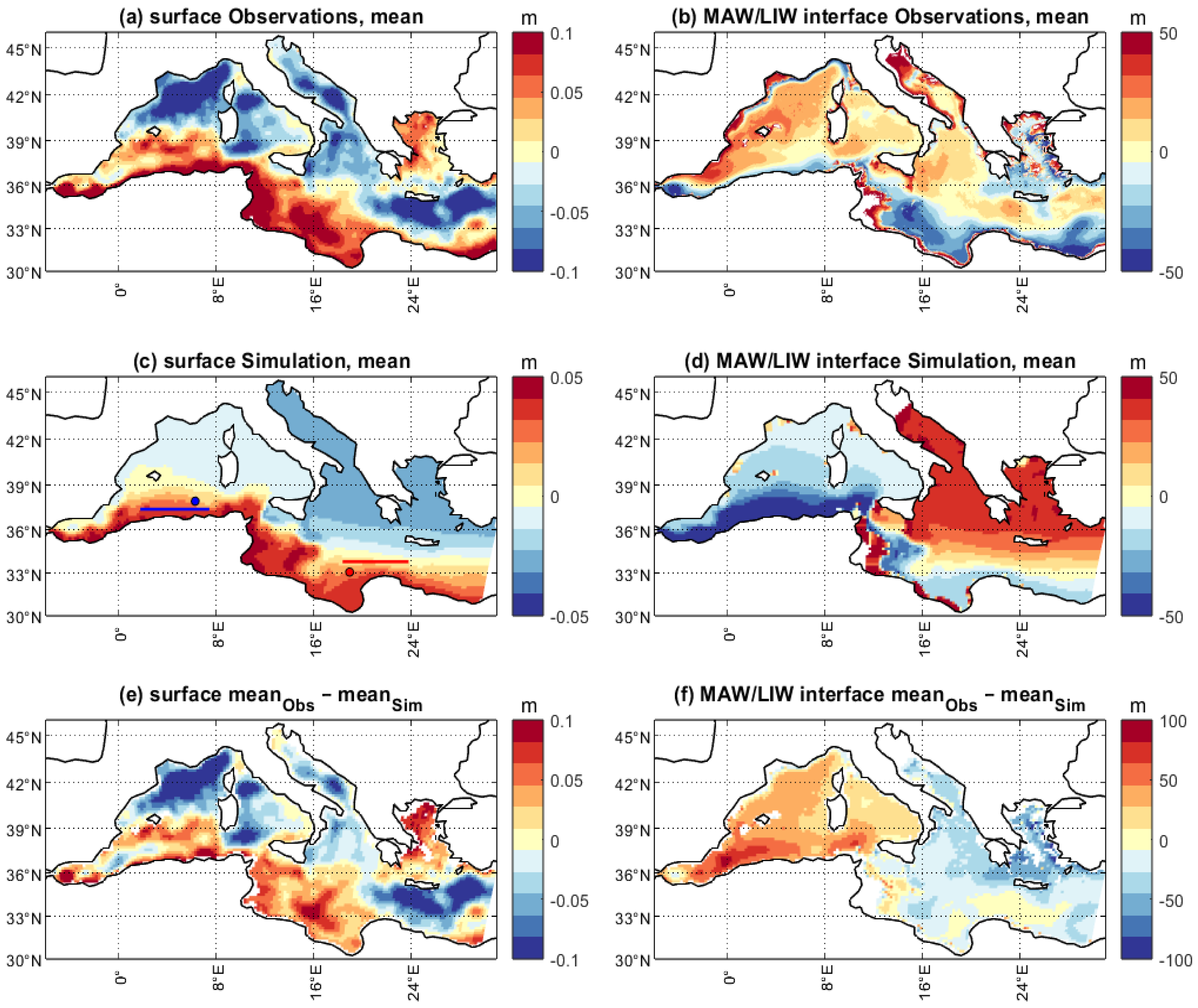
Remote-sensing observations of sea-surface height (SSH) over the Mediterranean Sea have been available since the TOPEX-Poseidon altimetric mission started in the early 1990s and, so far, they have allowed to characterize aspects of the local circulation up to interdecadal mean state and trends [45,46]. The SSH given by the ADT represents the streamfunction for the subsurface geostrophic current velocity and is therefore an invaluable parameter for investigating the near-surface circulation. The average SSH pattern (period 1993–2019, Figure 1a) shows several mesoscales as well as subbasin features, most of which have been investigated during the last two decades (see, e.g., refs. [11,47,48,49]). Noticeably, the field is dominated by a strong meridional gradient, particularly evident in the whole area located west of the Greek peninsula, consisting of higher SSH values in the proximity of the African coast and lower SSH values in the northern sub-basins. This pattern, which is a well-known, prominent, and persistent feature of Mediterranean SSH observations, clearly emerges even at shorter temporal scales (e.g., ref. [50]), and its origin, whether atmospherically forced or intrinsic, has never been investigated.
Less is known about the mean state and variability of the MAW/LIW interface. We use vertical profiles of seawater temperature and salinity to estimate the depth of the MAW/LIW interface from ocean reanalysis (see the Section 2) for the Mediterranean Sea (period 2001–2018, Figure 1b). The average anomalous pattern obtained after the removal of the spatial mean (around 93 m) is more complex than the SSH climatology, as it also reflects the underlying bathymetric features. Still, the pattern reveals a meridional gradient that mirrors (with opposite sign, as a consequence of baroclinic adjustment) the SSH pattern with lower elevations near the African coast and higher elevations at higher latitudes (the spatial average of the inferred MAW/LIW interface is at 148 m depth).
For both surface and intermediate layers, our simulation (Figure 1c,d) captures the main features of the observed climatological patterns, especially as far as the SSH is concerned, yielding spatial correlations and a spatial standard deviation that are 0.63 and 0.05 m, respectively, for the SSH patterns and 0.15 and 32.35 m, respectively, for the MAW/LIW patterns. The agreement is better in the southern portion of the basin, where the flow of MAW and LIW is known to be more intense and decreases northward. Noticeably, the agreement shows only small variations throughout the 300 years of the simulation, suggesting that the observed patterns contain robust stationary features of the Mediterranean IOV.
It is worth noting that, while intrinsic processes occurring in the world’s oceans are widely regarded as being the origin of a relevant part of the observed variability (the IOV, as already discussed), the authors are not aware of any attribution of the mean ocean state to intrinsic mechanisms that are, therefore, completely decoupled from the atmospheric action. In fact, even in model studies in which a constant-in-time or seasonally varying atmospheric forcing is used (a typical approach followed to reveal intrinsic oceanic processes), the mean ocean state is strongly affected by the surface momentum and heat fluxes [27,28,38].
Here, on the other hand, the peculiar boundary forcing adopted allows us to interpret the mean state represented by the SSH and MAW/LIW patterns (shown in Figure 1c,d, respectively) as the intrinsic oceanic response to the lateral input of energy and momentum, determined merely by the basin geometry and the baroclinic effects associated with the hydrological structure. Such a mean state, which we denote here as the “skeleton” of the Mediterranean Sea circulation, is –to our knowledge– the first case of an oceanic mean state that can be attributed to intrinsic mechanisms in which the atmosphere plays no role whatsoever. This is very relevant as far as the understanding of the Mediterranean Sea’s functioning and predictability are concerned. The difference between observed and simulated surface elevations (Figure 1e) and MAW/LIW interface positions (Figure 1f) can be ascribed, at least partly, to substantial differences in water stratification within the different layers (i.e., horizontal density gradients) through the basin, which are not considered in our study as they are strongly linked to atmospheric phenomena.
The long-term skeleton is clearly related to the geostrophic adjustment which characterizes the surface circulation of the southwestern part of the Mediterranean. However, its detailed shape is a non-trivial result of different elements. It cannot be evinced by simple considerations about the almost geostrophically adjusted state which has to characterize the surface circulation of the southwestern part of the Mediterranean Sea as far as its long-state equilibrium has to be achieved. Such equilibrium can be attained through different long-range transport shapes [51].
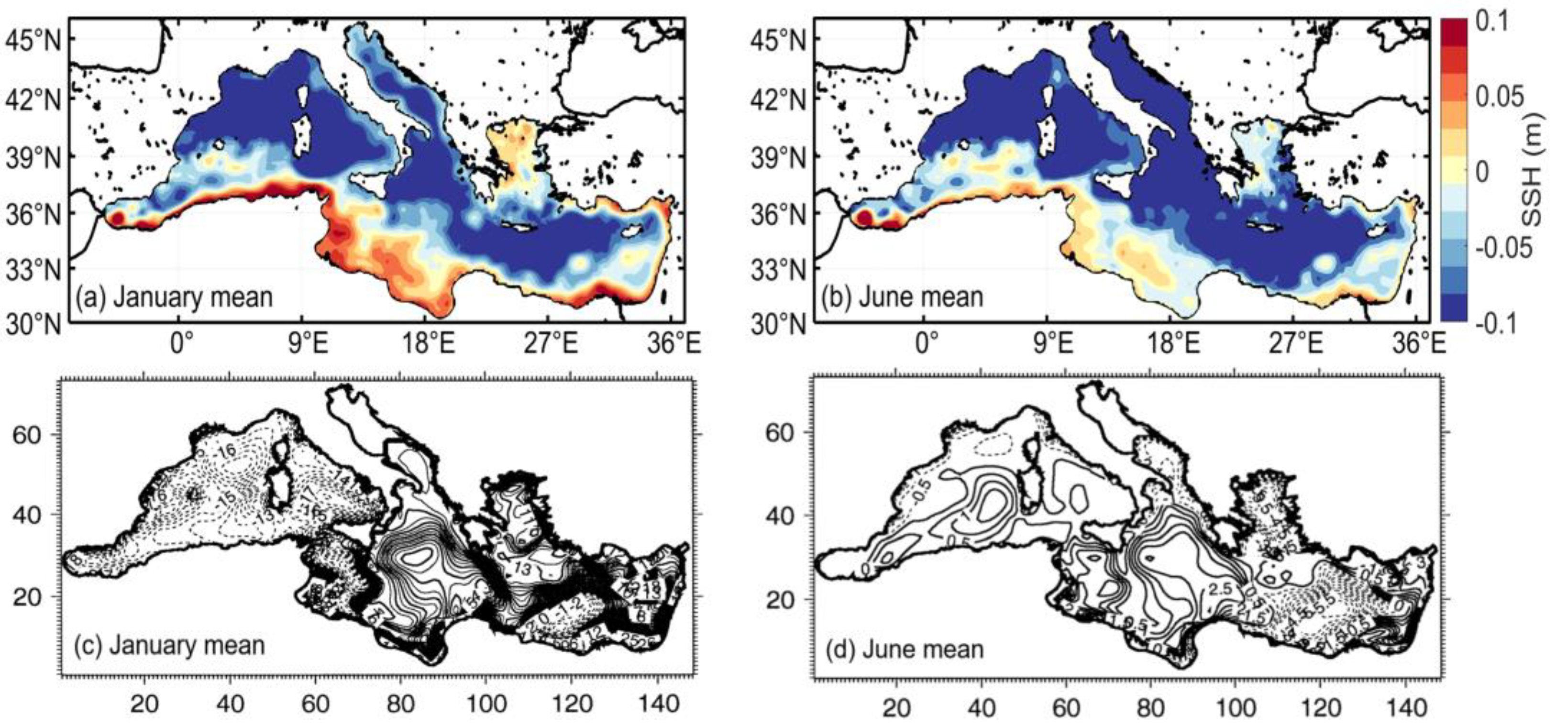
In addition to the reasonable model-data comparison (particularly significant for the SSH), evidence that our skeleton of Figure 1c prevails over the atmospheric forcing is obtained by considering the Mediterranean response to the surface wind stress for the months of January and June. Figure 2a shows the ADT averaged over the January months of the twenty-seven-year period under consideration. This map does not differ significantly from the mean state of Figure 1a, so its gross features are, again, in substantial agreement with the Mediterranean surface skeleton of Figure 1c.
Let us now compare Figure 2a with Figure 2c, which shows the modeled SSH averaged over the January months of an eight-year period obtained by Pierini and Simioli [15] by forcing a barotropic ocean model (in which, therefore, the baroclinic effects associated with MAW/LIW circulation are totally absent) with an interannual surface wind stress. Two main differences are evident: the negative SSH anomaly south of Sicily (corresponding to a cyclonic circulation) and the positive anomaly in the Ionian Sea south of the Italian peninsula (corresponding to an anticyclonic circulation) induced by the wind (Figure 2c) are opposite to those evidenced by the ADT (Figure 2a). One can therefore conclude that the Mediterranean surface skeleton prevails over the atmospherically induced circulation in those regions of the central Mediterranean. Similar conclusions can be drawn for the month of June (cfr. Figure 2b with Figure 2d).
3.2. The Intrinsic Variability
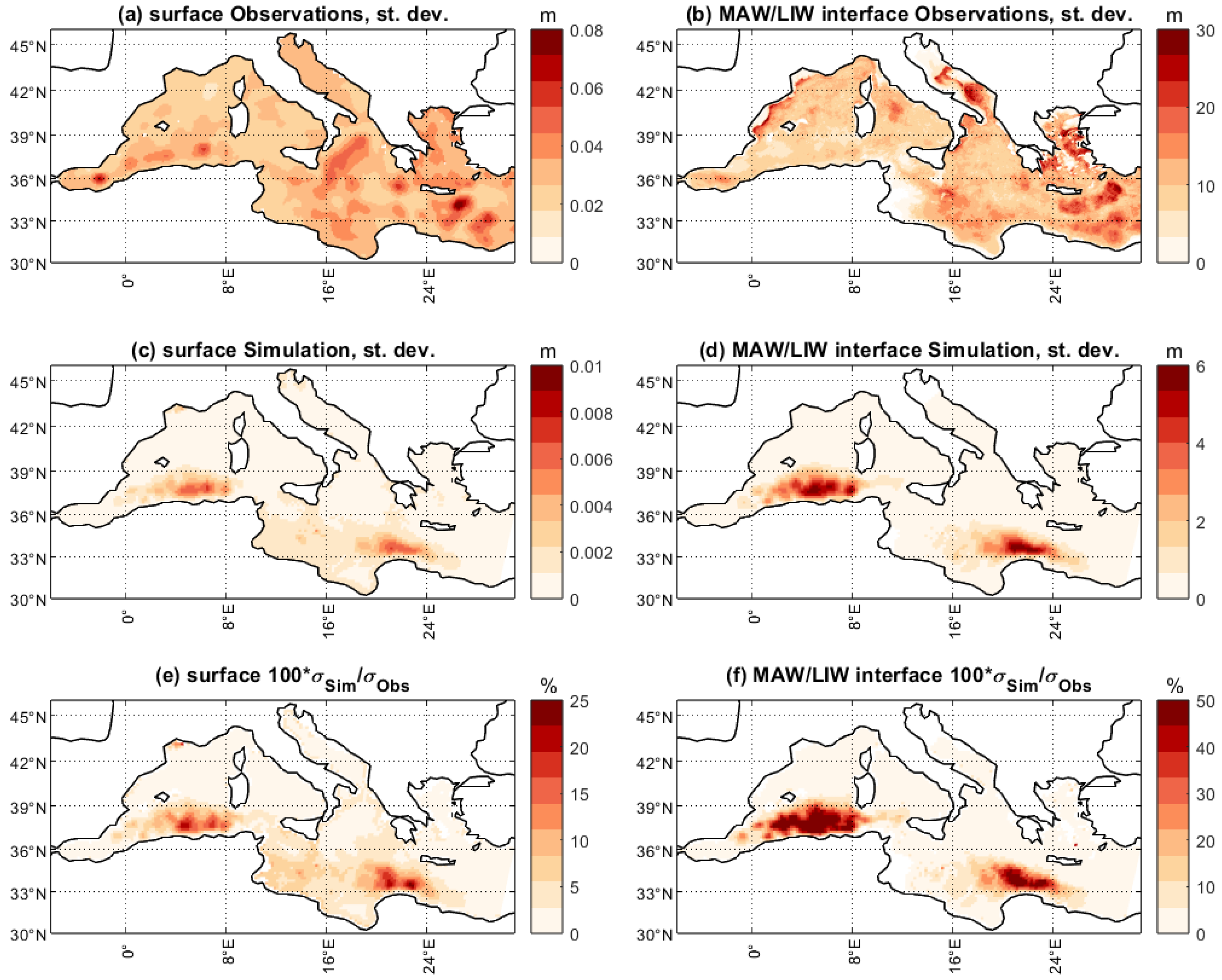
The spatial patterns of the local standard deviation of both the altimetric observations (Figure 3a) and MAW/LIW interface reanalysis (Figure 3b) reveal various regions of marked temporal variability, many of which correspond to well-known areas of strong mesoscale activity as far as SSH is concerned (e.g., refs. [49,52]), and to areas where strong interactions between intermediate flows and bathymetric features occur, as far as the MAW/LIW interface is concerned.
Our simulation (Figure 3c,d) yields patterns of marked variability as well, which are, again, to be ascribed solely to the Mediterranean IOV. Such variability is larger in regions where the flows of MAW and LIW are stronger, most noticeably west of the Strait of Gibraltar in the western basin and west of Crete in the eastern basin, while it is much weaker elsewhere. In large areas, mainly in the southern part of the basin, the amplitude of the simulated variability reaches around 20% of the observed variability at the surface (Figure 3e) and more than 50% in the interior layers (Figure 3f). Thus, the IOV appears to contribute significantly to the observed Mediterranean Sea variability.
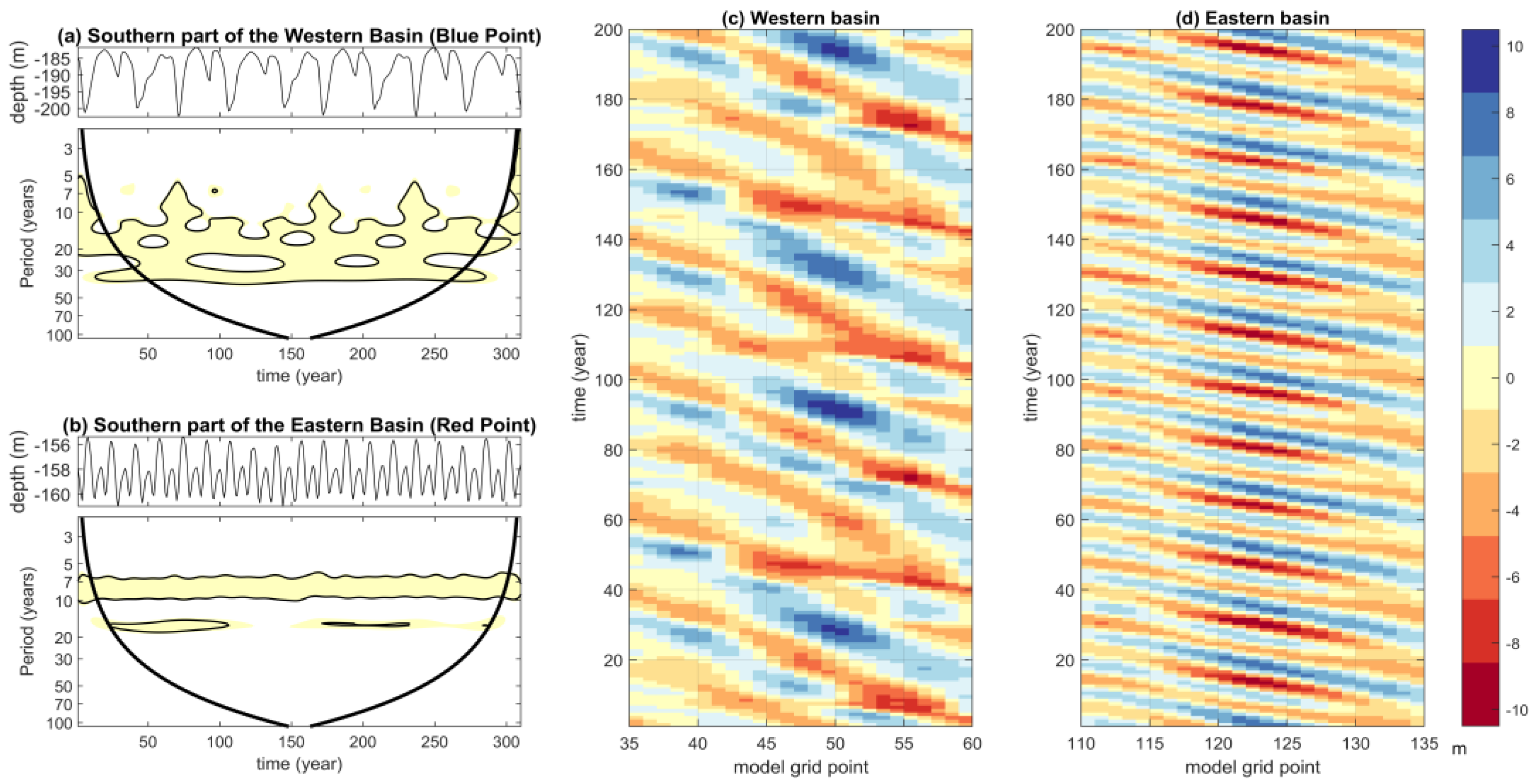
In the simulation, the IOV of the MAW/LIW interface yields self-sustained fluctuations within a well-defined range of interannual to multidecadal timescales for the Western Mediterranean (Figure 4a) and of interannual to decadal timescales for the Eastern Mediterranean (Figure 4b). To clarify the origin of such fluctuations, Figure 4c,d show the Hovmöller diagrams for the two zonal transects indicated in Figure 1c (blue and red lines) located in the core regions of MAW/LIW variability in the Western and Eastern Mediterranean sub-basins. The inclination of the isolines shows that, in both sub-basins, westward propagating waves are present; such inclination accounts for a phase speed of about 13.0 km/y in the western basin and 29.4 km/y in the eastern basin. In the simulation, the MAW/LIW variability is clearly baroclinic, as the surface and internal fluctuations are opposite in phase with those generated in the ocean interior (not shown).
4. Conclusions
In the present study, we have identified, for the first time, an intrinsic ocean mean state, which we have baptized as the “skeleton” of the Mediterranean Sea. This accounts for the well-known north-south SSH gradient visible in altimetric data—one of the most prominent and persistent features of Mediterranean surface observations—as the result of the Mediterranean intrinsic dynamics, which is shaped merely by the basing geometry and local hydrology rather than being the direct effect of atmospheric forcing.
The long-term skeleton is clearly related to the geostrophic adjustment which characterizes the surface circulation of the southwestern part of the Mediterranean. However, its detailed shape is a non-trivial result of different elements. It cannot be evinced by simple considerations about the almost geostrophically adjusted state which has to characterize the surface circulation of the southwestern part of the Mediterranean Sea as far as its long-state equilibrium has to be achieved. Such equilibrium can be attained through different long-range transport shapes.
A comparison between the altimetric ADT averaged over the months of January and June and the corresponding ocean response obtained by forcing a barotropic ocean model with interannual wind stress shows that the Mediterranean surface skeleton prevails over the atmospherically induced circulation in the central Mediterranean.
In addition, a strong and previously unknown IOV appears, which contributes to explaining a conspicuous part of the poorly understood observed interior low-frequency local oceanic variability. Indeed, self-sustained fluctuations of the MAW/LIW interface emerge within a well-defined range, spanning from interannual to multidecadal timescales in the Western Mediterranean and from interannual to decadal timescales in the Eastern Mediterranean.
These results pave the way to the identification and comprehension of the observed mean features and low-frequency fluctuations in oceanic datasets over the Mediterranean Sea as the result of intrinsic local processes. A similar modeling methodology could be adopted to explain fundamental dynamical features observed in other basins where lateral transports significantly contribute to shaping the local dynamics.
5. Data Availability
Annual mean absolute dynamic topography data for the period 1993–2019 are provided by the Copernicus Climate Data Store [40]. Original data have daily resolution.
Data from the Mediterranean MFC Physics Reanalysis for the period from 2004 to 2019 are provided by the Copernicus Marine Service [41].
6. Code Availability
Author Contributions
A.R. conceived the study, A.R. and D.Z. performed the numerical experiment, and A.R., S.P., S.R., D.Z. and M.G. analyzed the results. A.R., S.P., D.Z., M.G. and S.R. contributed to writing the paper. All authors have read and agreed to the published version of the manuscript.
Funding
This research received no external funding.
Institutional Review Board Statement
Not applicable.
Informed Consent Statement
Not applicable.
Data Availability Statement
Not applicable.
Acknowledgments
We would like to thank Peter Brandt and Richard J. Greatbatch for their helpful comments.
Conflicts of Interest
The authors declare no conflict of interest.
References
- Johnson, R.G. Climate control required a dam at the Strait of Gibraltar. Eos Trans. Am. Geophys. Union 1997, 78, 277–281. [Google Scholar] [CrossRef]
- Chan, W.-L. Effects of stopping the Mediterranean Outflow on the southern polar region. Polar Meteorol. Glaciol. 2003, 17, 25–35. [Google Scholar]
- Lozier, M.S.; Stewart, N.M. On the Temporally Varying Northward Penetration of Mediterranean Overflow Water and Eastward Penetration of Labrador Sea Water. J. Phys. Oceanogr. 2008, 38, 2097–2103. [Google Scholar] [CrossRef]
- Ivanovic, R.F.; Valdes, P.J.; Gregoire, L.; Flecker, R.; Gutjahr, M. Sensitivity of modern climate to the presence, strength and salinity of Mediterranean-Atlantic exchange in a global general circulation model. Clim. Dyn. 2014, 42, 859–877. [Google Scholar] [CrossRef]
- Ayache, M.; Swingedouw, D.; Colin, C.; Dutay, J.-C. Evaluating the impact of Mediterranean overflow on the large-scale Atlantic Ocean circulation using neodymium isotopic composition. Palaeogeogr. Palaeoclim. Palaeoecol. 2021, 570, 110359. [Google Scholar] [CrossRef]
- Bethoux, J.; Gentili, B.; Morin, P.; Nicolas, E.; Pierre, C.; Ruiz-Pino, D. The Mediterranean Sea: A miniature ocean for climatic and environmental studies and a key for the climatic functioning of the North Atlantic. Prog. Oceanogr. 1999, 44, 131–146. [Google Scholar] [CrossRef]
- Malanotte-Rizzoli, P.; Artale, V.; Borzelli-Eusebi, G.L.; Brenner, S.; Crise, A.; Gacic, M.; Kress, N.; Marullo, S.; Ribera d, M.; Sofianos, S.; et al. Physical forcing and physical/biochemical variability of the Mediterranean Sea: A review of un-resolved issues and directions for future research. Ocean Sci. 2014, 10, 281–322. [Google Scholar] [CrossRef]
- Rubino, A.; Gačić, M.; Bensi, M.; Kovačević, V.; Malačič, V.; Menna, M.; Negretti, M.E.; Sommeria, J.; Zanchettin, D.; Barreto, R.V.; et al. Experimental evidence of long-term oceanic circulation reversals without wind influence in the North Ionian Sea. Sci. Rep. 2020, 10, 1905. [Google Scholar] [CrossRef]
- Gačić, M.; Borzelli, G.L.E.; Civitarese, G.; Cardin, V.; Yari, S. Can internal processes sustain reversals of the ocean upper circulation? The Ionian Sea example. Geophys. Res. Lett. 2010, 37, L09608. [Google Scholar] [CrossRef]
- Gačić, M.; Ursella, L.; Kovačević, V.; Menna, M.; Malačič, V.; Bensi, M.; Negretti, M.-E.; Cardin, V.; Orlić, M.; Sommeria, J.; et al. Impact of dense-water flow over a sloping bottom on open-sea circulation: Laboratory experiments and an Ionian Sea (Mediterranean) example. Ocean Sci. 2021, 17, 975–996. [Google Scholar] [CrossRef]
- Brandt, P.; Rubino, A.; Quadfasel, D.; Alpers, W.; Sellschopp, J.; Fiekas, H.V. Evidence for the Influence of Atlantic–Ionian Stream Fluctuations on the Tidally Induced Internal Dynamics in the Strait of Messina. J. Phys. Oceanogr. 1999, 29, 1071–1080. [Google Scholar] [CrossRef]
- Rubino, A.; Zanchettin, D.; Androsov, A.; Voltzinger, N.E. Tidal Records as Liquid Climate Archives for Large-Scale Interior Mediterranean Variability. Sci. Rep. 2018, 8, 12586. [Google Scholar] [CrossRef] [PubMed]
- Zavatarielli, M.; Mellor, G.L. A Numerical Study of the Mediterranean Sea Circulation. J. Phys. Oceanogr. 1995, 25, 1384–1414. [Google Scholar] [CrossRef]
- Pinardi, N.; Korres, G.; Lascaratos, A.; Roussenov, V.; Stanev, E. Numerical simulation of the interannual variability of the Mediterranean Sea upper ocean circulation. Geophys. Res. Lett. 1997, 24, 425–428. [Google Scholar] [CrossRef]
- Pierini, S.; Simioli, A. A wind-driven circulation model of the Tyrrhenian Sea area. J. Mar. Syst. 1998, 18, 161–178. [Google Scholar] [CrossRef]
- Oddo, P.; Adani, M.; Pinardi, N.; Fratianni, C.; Tonani, M.; Pettenuzzo, D. A nested Atlantic-Mediterranean Sea general circulation model for operational forecasting. Ocean Sci. 2009, 5, 461–473. [Google Scholar] [CrossRef]
- Pinardi, N.; Coppini, G. Preface “Operational oceanography in the Mediterranean Sea: The second stage of development”. Ocean Sci. 2010, 6, 263–267. [Google Scholar] [CrossRef]
- Tsimplis, M.N.; Josey, S.A. Forcing of the Mediterranean Sea by atmospheric oscillations over the North Atlantic. Geophys. Res. Lett. 2001, 28, 803–806. [Google Scholar] [CrossRef]
- Zanchettin, D.; Rubino, A.; Traverso, P.; Tomasino, M. Teleconnections force interannual-to-decadal tidal variability in the Lagoon of Venice (northern Adriatic). J. Geophys. Res. Atmos. 2009, 114, D07106. [Google Scholar] [CrossRef]
- Criado-Aldeanueva, F.; Soto-Navarro, F.J.; García-Lafuente, J. Large-Scale Atmospheric Forcing Influencing the Long-Term Variability of Mediterranean Heat and Freshwater Budgets: Climatic Indices. J. Hydrometeorol. 2014, 15, 650–663. [Google Scholar] [CrossRef]
- Incarbona, A.; Martrat, B.; Mortyn, P.G.; Sprovieri, M.; Ziveri, P.; Gogou, A.; Jordà, G.; Xoplaki, E.; Luterbacher, J.; Langone, L.; et al. Mediterranean circulation perturbations over the last five centuries: Relevance to past Eastern Mediterranean Transient-type events. Sci. Rep. 2016, 6, 29623. [Google Scholar] [CrossRef]
- Cusinato, E.; Zanchettin, D.; Sannino, G.; Rubino, A. Mediterranean Thermohaline Response to Large-Scale Winter Atmospheric Forcing in a High-Resolution Ocean Model Simulation. Pure Appl. Geophys. 2018, 175, 4083–4110. [Google Scholar] [CrossRef]
- Dijkstra, H.A.; Ghil, M. Low-frequency variability of the large-scale ocean circulation: A dynamical systems approach. Rev. Geophys. 2005, 43, RG3002. [Google Scholar] [CrossRef]
- Pierini, S. A Kuroshio Extension System Model Study: Decadal Chaotic Self-Sustained Oscillations. J. Phys. Oceanogr. 2006, 36, 1605–1625. [Google Scholar] [CrossRef]
- Arbic, B.K.; Scott, R.B.; Flierl, G.R.; Morten, A.J.; Richman, J.G.; Shriver, J.F. Nonlinear Cascades of Surface Oceanic Geostrophic Kinetic Energy in the Frequency Domain. J. Phys. Oceanogr. 2012, 42, 1577–1600. [Google Scholar] [CrossRef]
- Arbic, B.K.; Müller, M.; Richman, J.G.; Shriver, J.F.; Morten, A.J.; Scott, R.B.; Sérazin, G.; Penduff, T. Geostrophic Turbulence in the Frequency–Wavenumber Domain: Eddy-Driven Low-Frequency Variability. J. Phys. Oceanogr. 2014, 44, 2050–2069. [Google Scholar] [CrossRef]
- Leroux, S.; Penduff, T.; Bessières, L.; Molines, J.-M.; Brankart, J.-M.; Sérazin, G.; Barnier, B.; Terray, L. Intrinsic and Atmospherically Forced Variability of the AMOC: Insights from a Large-Ensemble Ocean Hindcast. J. Clim. 2018, 31, 1183–1203. [Google Scholar] [CrossRef]
- Sérazin, G.; Penduff, T.; Barnier, B.; Molines, J.-M.; Arbic, B.K.; Müller, M.; Terray, L. Inverse Cascades of Kinetic Energy as a Source of Intrinsic Variability: A Global OGCM Study. J. Phys. Oceanogr. 2018, 48, 1385–1408. [Google Scholar] [CrossRef]
- Pierini, S.; Rubino, A. Modeling the Oceanic Circulation in the Area of the Strait of Sicily: The Remotely Forced Dynamics. J. Phys. Oceanogr. 2001, 31, 1397–1412. [Google Scholar] [CrossRef]
- Millot, C. The circulation of the Levantine Intermediate Water in the Algerian Basin. J. Geophys. Res. Ocean. 1987, 92, 8265–8276. [Google Scholar] [CrossRef]
- Malanotte-Rizzoli, P.; Manca, B.B.; Ribera, D.M.; Theocharis, A.; Bergamasco, A.; Bregant, D.; Budillon, G.; Civitarese, G.; Georgopoulos, D.; Michelato, A.; et al. A synthesis of the Ionian Sea hydrography, circulation and water mass pathways during PO-EM-Phase I. Prog. Oceanogr. 1997, 39, 153–204. [Google Scholar] [CrossRef]
- Millot, C. Circulation in the Western Mediterranean Sea. J. Mar. Syst. 1999, 20, 423–442. [Google Scholar] [CrossRef]
- Korres, G.; Pinardi, N.; Lascaratos, A. The Ocean Response to Low-Frequency Interannual Atmospheric Variability in the Mediterranean Sea. Part I: Sensitivity Experiments and Energy Analysis. J. Clim. 2000, 13, 705–731. [Google Scholar] [CrossRef]
- Rubino, A.; Romanenkov, D.; Zanchettin, D.; Cardin, V.; Hainbucher, D.; Bensi, M.; Boldrin, A.; Langone, L.; Miserocchi, S.; Turchetto, M. On the descent of dense water on a complex canyon system in the southern Adriatic basin. Cont. Shelf Res. 2012, 44, 20–29. [Google Scholar] [CrossRef]
- Hessner, K.; Rubino, A.; Brandt, P.; Alpers, W. The Rhine Outflow Plume Studied by the Analysis of Synthetic Aperture Radar Data and Numerical Simulations. J. Phys. Oceanogr. 2001, 31, 3030–3044. [Google Scholar] [CrossRef]
- Rubino, A.; Hessner, K.; Brandt, P. Decay of Stable Warm-Core Eddies in a Layered Frontal Model. J. Phys. Oceanogr. 2002, 32, 188–201. [Google Scholar] [CrossRef]
- National Geophysical Data Center. ETOPO2v2 2 Minute Worldwide Bathymetry/Topography Grids|NCEI. Available online: https://www.ngdc.noaa.gov/mgg/fliers/06mgg01.html (accessed on 4 October 2023).
- Penduff, T.; Llovel, W.; Close, S.; Garcia-Gomez, I.; Leroux, S. Trends of Coastal Sea Level Between 1993 and 2015: Imprints of Atmospheric Forcing and Oceanic Chaos. Surv. Geophys. 2019, 40, 1543–1562. [Google Scholar] [CrossRef]
- Carret, A.; Llovel, W.; Penduff, T.; Molines, J. Atmospherically Forced and Chaotic Interannual Variability of Regional Sea Level and Its Components Over 1993–2015. J. Geophys. Res. Oceans 2021, 126, e2020JC017123. [Google Scholar] [CrossRef]
- Lopez, A. Sea Level Daily Gridded Data from Satellite Observations for the Mediterranean Sea from 1993 to 2020. 2018. Available online: https://cds.climate.copernicus.eu/cdsapp#!/dataset/satellite-sea-level-mediterranean?tab=overview (accessed on 4 October 2023).
- Escudier, R.; Clementi, E.; Omar, M.; Cipollone, A.; Pistoia, J.; Aydogdu, A.; Drudi, M.; Grandi, A.; Lyubartsev, V.; Lecci, R.; et al. Mediterranean Sea Physical Reanalysis (CMEMS MED-Currents, E3R1 System). Copernicus Monitoring Environment Marine Service (CMEMS), 2020. Available online: https://data.marine.copernicus.eu/product/MEDSEA_MULTIYEAR_PHY_006_004/description?view=-&product_id=-&option=- (accessed on 4 October 2023).
- Torrence, C.; Compo, G. A practical guide to wavelet analysis. Bull. Am. Meteorol. Soc. 1998, 79, 61–78. [Google Scholar] [CrossRef]
- Grinsted, A.; Moore, J.C.; Jevrejeva, S. Application of the cross wavelet transform and wavelet coherence to geophysical time series. Nonlinear Process. Geophys. 2004, 11, 561–566. [Google Scholar] [CrossRef]
- Zanchettin, D.; Rubino, A.; Jungclaus, J.H. Intermittent multidecadal-to-centennial fluctuations dominate global temperature evolution over the last millennium. Geophys. Res. Lett. 2010, 37, L14702. [Google Scholar] [CrossRef]
- Wilson, W.S.; Lindstrom, E.J.; Willis, J.K. Satellite Oceanography—History and Introductory Concepts. In Encyclopedia of Ocean Sciences, 3rd ed.; Cochran, J.K., Bokuniewicz, H.J., Yager, P.L., Eds.; Academic Press: Cambridge, MA, USA, 2019; pp. 347–361. [Google Scholar] [CrossRef]
- Zanchettin, D.; Bruni, S.; Raicich, F.; Lionello, P.; Adloff, F.; Androsov, A.; Antonioli, F.; Artale, V.; Carminati, E.; Ferrarin, C.; et al. Sea-level rise in Venice: Historic and future trends (review article). Nat. Hazards Earth Syst. Sci. 2021, 21, 2643–2678. [Google Scholar] [CrossRef]
- Malanotte-Rizzoli, P.; Manca, B.B.; D’Alcala, M.R.; Theocharis, A.; Brenner, S.; Budillon, G.; Ozsoy, E. The Eastern Mediterranean in the 80s and in the 90s: The big transition in the intermediate and deep circulations. Dyn. Atmos. Oceans 1999, 29, 365–395. [Google Scholar] [CrossRef]
- Larnicol, G.; Ayoub, N.; Le Taron, P.Y. Major changes in Mediterranean Sea level variability from 7 years of TOPEX/Poseidon and ERS-1/2 data, Major changes in Mediterranean Sea level variability from 7 years of TOPEX/Poseidon and ERS-1/2 data. J. Mar. Syst. 2002, 33–34, 63–89. [Google Scholar] [CrossRef]
- Menna, M.; Suarez, N.R.; Civitarese, G.; Gačić, M.; Rubino, A.; Poulain, P.-M. Decadal variations of circulation in the Central Mediterranean and its interactions with mesoscale gyres. Deep. Sea Res. Part II Top. Stud. Oceanogr. 2019, 164, 14–24. [Google Scholar] [CrossRef]
- Rio, M.-H.; Mulet, S.; Picot, N. Beyond GOCE for the ocean circulation estimate: Synergetic use of altimetry, gravimetry, and in situ data provides new insight into geostrophic and Ekman currents. Geophys. Res. Lett. 2014, 41, 8918–8925. [Google Scholar] [CrossRef]
- Dengler, M.; Schott, F.A.; Eden, C.; Brandt, P.; Fischer, J.; Zantopp, R.J. Break-up of the Atlantic deep western boundary current into eddies at 8° S. Nature 2004, 432, 1018–1020. [Google Scholar] [CrossRef]
- Pujol, M.-I.; Larnicol, G. Mediterranean sea eddy kinetic energy variability from 11 years of altimetric data. J. Mar. Syst. 2005, 58, 121–142. [Google Scholar] [CrossRef]
- Pawlowicz, R. M_Map: A Mapping Package for Matlab. University of British Columbia Earth and Ocean Sciences. 2020. Available online: http://www.eos.ubc.ca/rich/map.html (accessed on 4 October 2023).
- Wessel, P.; Smith, W.H. A global, self-consistent, hierarchical, high-resolution shoreline database. J. Geophys. Res. Solid Earth 1996, 101, 8741–8743. [Google Scholar] [CrossRef]
Figure 1.
Comparison between the mean state of the Mediterranean SSH (left panels) and of the depth of the MAW/LIW interface (right panels) from observations (top panels, from the ADT provided by the Copernicus satellite data for the period 1993–2019 and from an ocean reanalysis for the period 2001–2018, respectively) and from simulations (mid panels, from a multi-centennial ocean model simulation obtained by imposing a steady lateral forcing without any atmospheric forcing). Data are annual average elevations (panels (a,c)) and annual average anomalies (panels (b,d)) from the spatial mean plotted on the original grids. In panel (c), the red and blue dots indicate the position where a wavelet analysis was performed; the two lines indicate the sections considered for the Hovmöller diagrams. Panels (e,f) show the differences between observed and simulated mean SSH and interface position.

Figure 2.
Comparison between the altimetric ADT averaged over the months of January (panel (a)) and June (panel (b)) and the ocean response, averaged over the same months (panels (c,d)) of an eight-year period by forcing a barotropic ocean model with an interannual wind stress field (continues and dashed lines indicate positive and negative values, respectively; the two panels are adapted from the same article). Panels (c,d) adapted with permission from Pierini and Simioli [15] (1998, Journal of Marine Systems).

Figure 3.
Top and mid panels: as in Figure 1 but for the local standard deviation. Bottom panels: the ratio between the standard deviation of simulated and the observed data (in %); high values indicate regions where the IOV contributes significantly to the observed variability.
Figure 3.
Top and mid panels: as in Figure 1 but for the local standard deviation. Bottom panels: the ratio between the standard deviation of simulated and the observed data (in %); high values indicate regions where the IOV contributes significantly to the observed variability.

Figure 4.
Time series and wavelet of the modeled MAW/LIW interface sampled at the two sites indicated in Figure 1c (blue and red dots) in the southern Western (panel (a)) and Eastern (panel (b)) Mediterranean Sea, where the simulated IOV is strong. Hovmöller diagrams of the IOV of the MAW-LIW interface (model level 5) sampled along the transects shown in Figure 1c (blue and red lines) and averaged between five meridional grid points in the Western Mediterranean (panel (c)) and in the Eastern Mediterranean (panel (d)). The inclination of the isolines indicates westward propagation. Data are anomalies from the local climatology.

Disclaimer/Publisher’s Note: The statements, opinions and data contained in all publications are solely those of the individual author(s) and contributor(s) and not of MDPI and/or the editor(s). MDPI and/or the editor(s) disclaim responsibility for any injury to people or property resulting from any ideas, methods, instructions or products referred to in the content. |
© 2023 by the authors. Licensee MDPI, Basel, Switzerland. This article is an open access article distributed under the terms and conditions of the Creative Commons Attribution (CC BY) license (https://creativecommons.org/licenses/by/4.0/).
Share and Cite
MDPI and ACS Style
Rubino, A.; Pierini, S.; Rubinetti, S.; Gnesotto, M.; Zanchettin, D. The Skeleton of the Mediterranean Sea. J. Mar. Sci. Eng. 2023, 11, 2098. https://doi.org/10.3390/jmse11112098
AMA Style
Rubino A, Pierini S, Rubinetti S, Gnesotto M, Zanchettin D. The Skeleton of the Mediterranean Sea. Journal of Marine Science and Engineering. 2023; 11(11):2098. https://doi.org/10.3390/jmse11112098
Chicago/Turabian StyleRubino, Angelo, Stefano Pierini, Sara Rubinetti, Michele Gnesotto, and Davide Zanchettin. 2023. "The Skeleton of the Mediterranean Sea" Journal of Marine Science and Engineering 11, no. 11: 2098. https://doi.org/10.3390/jmse11112098
Note that from the first issue of 2016, this journal uses article numbers instead of page numbers. See further details here.