Article

Bayesian Network Analysis for Shoreline Dynamics, Coastal Water Quality, and Their Related Risks in the Venice Littoral Zone, Italy

by
Hung Vuong Pham
1,2,
Maria Katherina Dal Barco
1,2,
Mohsen Pourmohammad Shahvar
1,
Elisa Furlan
1,2,
Andrea Critto
1,2,* and
Silvia Torresan
1,2
1
Department of Environmental Sciences, Informatics and Statistics, Ca’ Foscari University of Venice, 30171 Venice, Italy
2
Risk Assessment and Adaptation Strategies Division, Fondazione Centro Euro-Mediterraneo sui Cambiamenti Climatici, 30121 Venice, Italy
*
Author to whom correspondence should be addressed.
J. Mar. Sci. Eng. 2024, 12(1), 139; https://doi.org/10.3390/jmse12010139
Submission received: 29 November 2023 / Revised: 4 January 2024 / Accepted: 7 January 2024 / Published: 10 January 2024
(This article belongs to the Special Issue Sea Level Rise and Related Hazards Assessment)

Abstract

:
The coastal environment is vulnerable to natural hazards and human-induced stressors. The assessment and management of coastal risks have become a challenging task, due to many environmental and socio-economic risk factors together with the complex interactions that might arise through natural and human-induced pressures. This work evaluates the combined effect of climate-related stressors on low-lying coastal areas by applying a multi-risk scenario analysis through a Bayesian Network (BN) approach for the Venice coast. Based on the available open-source and remote sensing data for detecting shoreline changes, the developed BN model was trained and validated with oceanographic variables for the 2015–2019 timeframe, allowing us to understand the dynamics of local-scale shoreline erosion and related water quality parameters. Three “what-if” scenarios were carried out to analyze the relationships between oceanographic boundary conditions, shoreline evolution, and water quality parameters. The results demonstrate that changes in sea surface height and significant wave height may significantly increase the probability of high-erosion and high-accretion states. Moreover, by altering the wave direction, the water quality variables show significant changes in the higher-risk class. The outcome of this study allowed us to identify current and future coastal risk scenarios, supporting local authorities in developing adaptation plans.

1. Introduction

Coastal regions are distinct and delicate ecosystems, influenced by complex and dynamic interactions among various physical, ecological, and socio-economic elements at the boundary between land and sea [1,2,3,4,5]. They are susceptible both to acute and chronic hazards stemming from climate variability [6,7,8]. The primary challenges arise from sea level rises and intensified waves and storm surges. These factors can cause land loss, coastal erosion, flooding, and changes in the physical–chemical properties of seawater (temperature, salinity, nutrients, pH, oxygen, etc.), affecting biodiversity and ecosystem services in coastal waters [9].
Coastal erosion is primarily driven by physical factors, like wave, wind, current, and subsidence [10,11,12,13,14,15]. This phenomenon occurs when there is a negative long-term balance in sediment dynamics, meaning that sediment removal surpasses deposition. Regions with low elevation and flat topography, such as the Netherlands and the Po Valley in Italy, are especially vulnerable to these impacts.
In recent years, human activities have significantly escalated the problem related to coastal erosion [14,16]. Actions along coastlines, like harbor constructions, aquaculture, and land reclamation, coupled with activities within river basins, such as river diversions and damming, as well as offshore actions like seafloor dredging and sand extraction, frequently intensify coastal erosion.
In some regions, new areas prone to erosion may arise as a consequence of climate change and the subsequent rise in sea levels [9,17,18]. Sea level rise can lead to the permanent flooding of coastal zones, intensifying the repercussions of coastal erosion and storm-related flooding [19]. Given these challenges, it is essential to have accurate assessments of coastal erosion to inform Integrated Coastal Zone Management (ICZM) strategies and climate change adaptation measures [20]. Such assessments are necessary to aid international, national, and local stakeholders and communities in navigating the impacts of climate change, proactively identifying potential environmental degradation and mitigating associated financial losses [21].
Accurate assessments of coastal erosion require comprehensive data about historical and projected shoreline positions. Such information is crucial for devising coastal protection strategies, evaluating the risks posed by sea level rises and storm surges and fine-tuning modeling predictions [22]. Nowadays, remote sensing emerges as a pivotal tool for monitoring coastal regions, offering diverse spatial and temporal resolutions [23]. The advantages of remote sensing data are manifold, encompassing their ability to furnish affordable, consistent, and precise data, even for inaccessible regions. Within these techniques, the analysis of satellite imagery stands out as a cost-effective and rapid approach for tracking shoreline shifts over time [24,25,26,27]. In particular, infrared and multi-spectral satellite images hold significant promise in effectively recognizing the land–water interface [28].
The rapid evolution and deployment of satellite imagery in recent decades have empowered the scientific community to devise innovative methodologies for harnessing remote sensing data to their fullest potential. In this context, Machine Learning (ML) approaches have become increasingly utilized for environmental studies in different contexts and applications, such as forecasting and modeling, characterization of hazards, detection of potential exposure and vulnerability, and risk assessment [29]. Among ML methods, sophisticated probabilistic-based methods, known as Bayesian Networks (BNs), have been developed, allowing for integration into a single model of heterogeneous information (e.g., remote sensing data, physical, chemical data, ecosystem services, and expert judgment), providing useful insights for managers and decision makers in designing adaptation strategies [30,31,32]. Several reviews on the application of the BN models highlighted the increased use of this probabilistic model for environment risk assessment due to their capability to cooperate joint probability distribution to examine the potential impacts of numerous risk factors and stressors for assessment endpoints under baseline conditions and future projections [32,33,34]. In particular, BN applications have been implemented to assess coastal risk, linked to specific stressors, including storm surges’ vulnerability against environmental and human receptors [35]. On the other hand, BNs have also been designed for risk management and assessment to appraise the effectiveness of adaptation or management strategies to understand the level of risk or adverse conditions. For instance, Ref. [36] integrated the assessment of adaptation measures and prediction of the SLR-induced coastal erosion into the GIS-based BN model.
Building upon the stated objective, this research centered on evaluating the risk of coastal erosion for the coastal line of Venice (hereafter refer to as Venice case study), including Pellestrina, Lido, and Cavallino. To reach this aim, the Bayesian Network approach was implemented to assess the effect of sea level rises on coastal erosion and water quality risks under different “what-if” scenarios related to extreme oceanographic conditions (i.e., sea level, wave, wind wave height, and direction).

2. Materials and Methods
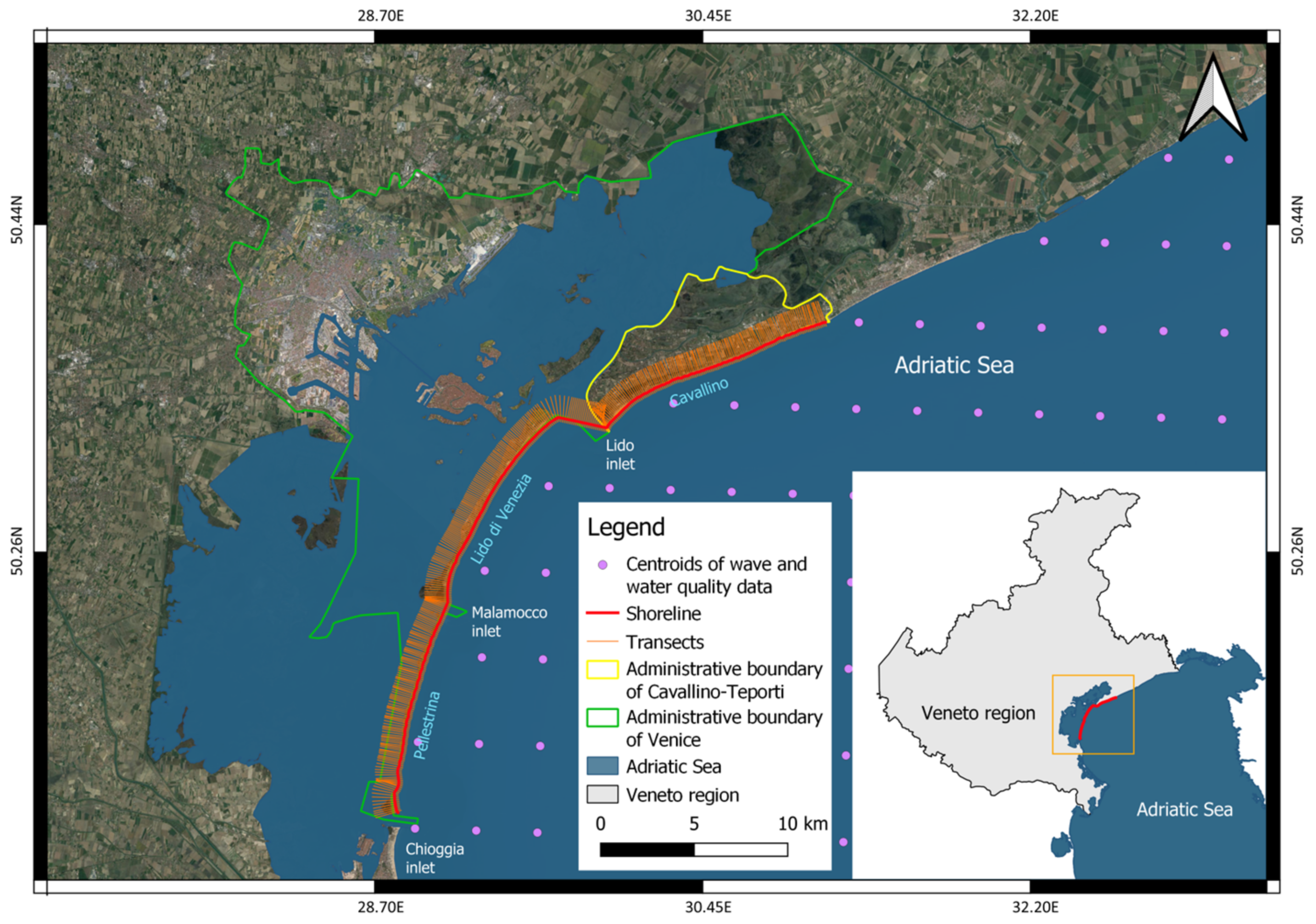
2.1. Case Study

The Venice case study encompasses the coastline of two islands, namely Pellestrina, Lido, and the coast of Cavallino peninsula (Figure 1). Spanning approximately 90 km, this coastline is characterized by gentle-sloping and shallow sandy littorals where sediments originate from Tagliamento, Piave, Sile, Brenta, and Adige rivers [37]. This coast acts as a barrier to separate the Venice Lagoon and the Adriatic Sea.
Since the study area is situated at the land–sea boundary, it is particularly vulnerable due to its diverse morphological features, including straight coastlines, lagoon barrier islands, spits, river estuaries [38,39,40], and numerous human-induced stressors. Additionally, anthropogenic activities, like the construction of coastal defenses, breakwaters, and the construction of the Experimental Electromechanical Module—MoSE project [41,42], have further impacted the morphology of the Venice coastline [37,43,44]. Furthermore, the Venice shoreline is particularly vulnerable to extreme sea levels due to various factors, such as astronomical tides, storm surges, and relative sea level rises [18,45,46,47]. Particularly, waves primarily originate from two prevailing wind directions, namely, southeast (Sirocco wind) and northeast (Bora wind). Significant wave height demonstrated a yearly cycle with a peak from November to March (e.g., from 2 to 4 m in the winter months) [48]. The wave direction is mainly determined by bora wind (northeast to southwest) while the peak waves are found more frequently with the sirocco regime (southeast to northwest) [48].
Together with storm surges and sea level rise, the subsidence of the territory contributes to the increased frequency of flooding events (i.e., so-called “acqua alta” in Italian) such as recorded flood events in 1966 and 2019. The subsidence in the North Adriatic region results from both natural (e.g., tectonics, glacio-isostasy, and compaction of alluvial fine-material deposits) and anthropogenic factors, notably groundwater extraction, acting at different time scales [49,50]. Combining both subsidence and the impacts of climate change, the relative sea level rise has been increasing in this region at a rate of 1.2 mm.year−1 for the timeframe 1872–2019 [46,51], and this is expected to keep rising in the future [18,47,52]
Given these compounding stressors, the case study area is projected to suffer an increased risk of flooding and shoreline retreatment [53], losses, and potential alterations to barrier islands like Lido and Pellestrina, thus exacerbating flood threats to Venice’s historic center and its surrounding lagoon [54]. Several solutions have been implemented to cope with these problems, such as beach nourishment in Pellestrina and Cavallino-Treporti, rubble-mound seawalls, and submerged breakwater along the coast [55]. Moreover, some nature-based solutions have been carried out during the LIFE SeResto (http://www.lifeseresto.eu/, accessed on 17 December 2022) and LIFE ReDune (http://www.liferedune.it/, accessed on 17 December 2022) projects to expand dune vegetation, wetlands, and seagrasses in the Venice lagoon, aiming at restoring increasing the resilience of coastal-lined lagoon habitats to flooding and erosion [56]. However, further actions are needed to better understand, prepare for, and manage climate risks and help accelerate the adoption of comprehensive adaptation plans and approaches at the regional to local scale, as required by the EU Adaptation Strategy 2021 [57].

2.2. Input Data

For better understanding and managing coastal risks, including those related to climate change such as shoreline erosion and water quality variations, it is necessary to collect heterogeneous data concerning the territorial and environmental features of the study area (e.g., satellite images, tide levels, water quality parameters) and the oceanographic drivers (e.g., wave and wind characteristics) acting on the coast. Conceptually, the BN application requires data for the causal nodes (or parent nodes) at the top of the model and the effect nodes (or child nodes) at the bottom of the model [58]. In this application, the parent nodes contain the main stressor or cause variables, such as wave, wind-wave, and current parameters, while the child nodes or effect nodes are the final assessment endpoints, namely water quality and shoreline change. All the above-mentioned data were collected from freely available data sources, including the Copernicus Marine Service (CMEMS) and the Earth Explorer platform (https://earthexplorer.usgs.gov/, accessed on 19 August 2022). Based on the availability of these open data, the timeframe 2015–2019 was selected as the study period since the satellite images from Sentinel-2 data were released in June 2015. A list of selected variables, together with their abbreviations used in this work and their metadata, is reported in Table 1.
The selected variables are divided into 3 main groups, namely, oceanographic parameters, water quality, and shoreline change. The first 2 groups were obtained from the CMEMS platform, while the shoreline evolution (SEV), representing the historical trend of the coastline (i.e., accretion, stability, and erosion), was taken from [59].
Regarding the CMEMS dataset, oceanographic and water quality data were retrieved to identify the main stressors of coastal erosion processes and to identify potential targets. These data were obtained in the NetCDF format with different resolutions, i.e., about 6 km for the variables related to the current and about 4 km for the ones related to wave, wind, and water quality. As highlighted in many works, the shoreline changes are driven by both cross-shore and longshore processes [60,61]. The former is mainly governed by the wave parameters (i.e., direction, period, and height), while the latter is controlled primarily by the current and its velocity [61]. Therefore, the set of data obtained from CMEMS provides a wide range of variables to understand the evolution of the shoreline, the associated sediment transport process, and, consequently, water quality parameters.
For analyzing shoreline changes, several ML techniques were employed. Specifically, Logistic Regression [62], Neural Networks [63], and Random Forest [64] algorithms were utilized to detect the shoreline (i.e., the delineation between land and sea), based on the selected satellite images in the reference scenario 2015–2019 [59]. Then, the Digital Shoreline Evolution System (DSAS) was utilized to estimate the annual changing rate (i.e., Net Shoreline Movement—NSM) for all transects along the coast (i.e., perpendicular segments intersecting each shoreline at regular spatial distance, as shown in Figure 1). Nevertheless, the collection of satellite images to carry out the shoreline evolution analysis was limited due to the availability of data related to the spatial resolution, cloud cover, and the consistency in tidal level, which does not allow for the seasonal assessment. Considering the spatial coverage of the case study, transects were established at distance of 100 m to ensure comprehensive coverage while maintaining a manageable calculation time. The outcomes of this analysis are maps of yearly shoreline changes for the timeframe 2015–2019 with a spatial resolution of 100 m along the coast.

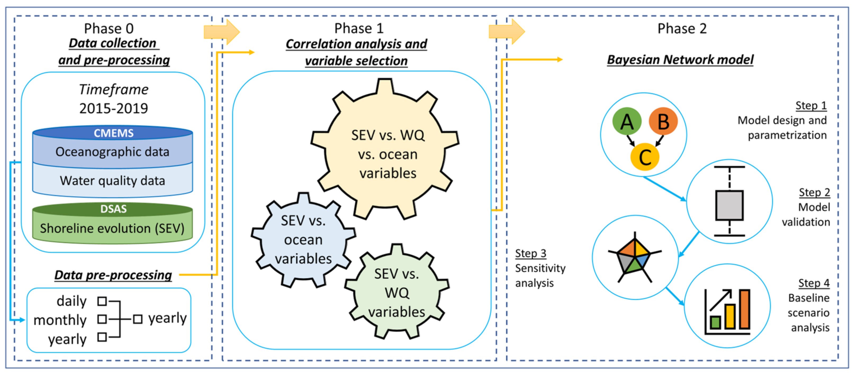
2.3. Methodological Approach

This section presents the Bayesian Network approach adopted for the analysis of coastal risks for the Venice littoral in the reference scenario 2015–2019. In particular, the dynamic evolution of the shoreline leads to cascading effects on both human (i.e., lives, activities, and infrastructure) and natural systems (e.g., water quality deterioration due to the rising of turbidity) [65,66].
As emerged from recent literature reviews, BN models are increasingly being used for environmental risk assessment [32,33,34] for different assessment endpoints (e.g., water quality, biological invasion, ecological status, coastal erosion) and purposes (e.g., impact assessment, scenario analysis) in various environmental domains, such as freshwater, marine, terrestrial, and urban area. For this kind of application, most of the BN studies are expert systems. Moreover, the model structure typically evolves a synthesis of pre-existing models, combined with insights from experts and stakeholders [34].
As presented in Figure 2, the assessment builds on the results of the shoreline evolution trend analysis of satellite images and the data obtained from CMEMS, as summarized in Table 1, and follows a stepwise approach that allows for estimating risk scenarios for the three assessment endpoints, namely, shoreline evolution (SEV), suspended particulate matter (SPM), and diffuse attenuation (KD).
Specifically, after the preliminary data collection and pre-processing (Phase 0), the correlation analysis and variable selection (Phase 1) were carried out to reduce the complexity of the BN model by identifying high-correlated variables in three different settings: (i) correlation among selected variables; (ii) sub-matrix including SEV against its physical oceanographic drivers; (iii) sub-matrix including the SEV and water quality variables. Then, the development of the BN model (Phase 2) followed different steps, including (i) model design and parameterization; (ii) model validation; (iii) sensitivity analysis; and (iv) the baseline scenario analysis.

2.3.1. Phase 0: Data Collection and Pre-Processing

As shown in Figure 2, the main goal of this initial phase is to elaborate and homogenize the grid-based dataset (i.e., oceanographic and water quality data) retrieved from the Copernicus CMEMS portal and the transect-based data (i.e., shoreline evolution). Moreover, the input data have different temporal resolutions, i.e., hourly records for oceanographic variables and monthly data for the sea surface height, current, and water quality parameters (i.e., KD and SPM). Therefore, to be implemented into the BN model, input data were pre-processed in Climate Data Operators (CDOs) [67], calculating a yearly mean value, as well as the maximum value only for certain variables (i.e., WAH and WIH) to capture extreme events through the investigated timeframe. Given the diverse formats and spatiotemporal resolutions of the input data, they are uniformly converted into a yearly basis and extracted at the central point of the shoreline transects to build a comprehensive table to train the BN model. This integration strategy served the purpose of homogenizing the data, thereby mitigating the potential inconsistencies and biases that could influence the final findings. The resulting table is composed of 12 columns, where each of them represents a selected variable, including the final assessment endpoints in the last 3 columns.

2.3.2. Phase 1: Correlation Analysis and Variable Selection

Once the pre-processing phase was completed, the correlation analysis was carried out to identify the high-correlated variables of the collected dataset whilst reducing the complexity of the BN model. Specifically, the correlation table and the plot report the relationships and possible dependencies among shorelines, water quality, and oceanographic variables. The ‘PerformanceAnalytics’ package from the open-source R program was selected to perform the statistical analysis and obtain the graphical outputs, facilitating the understanding of the results. The resulting outcome is a matrix with a dimension equal to the number of variables considered in the data pre-processing phase (see Table 1) and will be discussed in Section 3.1. The correlation matrix reports the correlation coefficient, with −1 denoting a perfectly negative correlation between the considered variables, 0 signifying no correlation between the variables, and 1 indicating a perfect positive correlation between the variables.

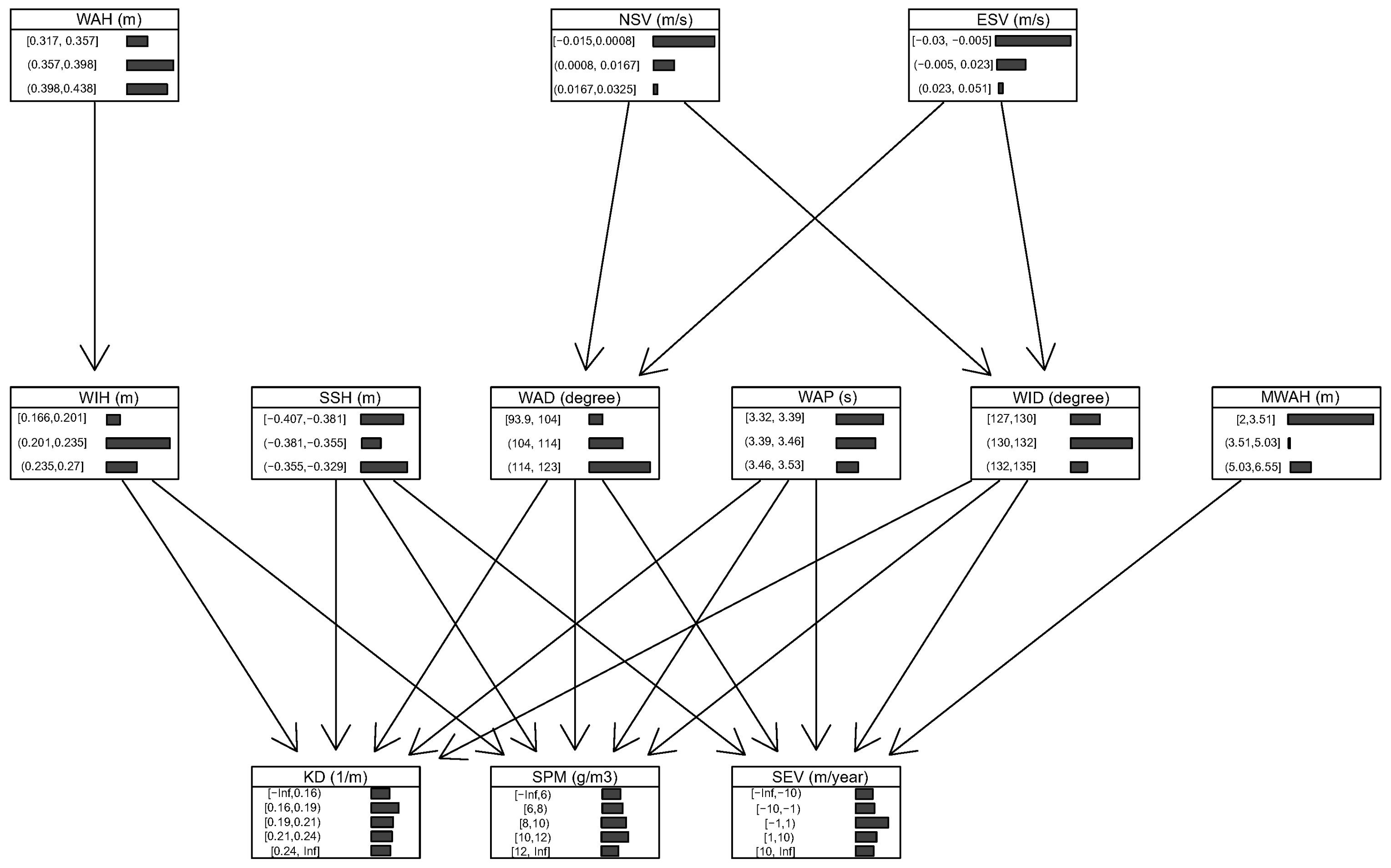
2.3.3. Phase 2: Bayesian Network Model

The final phase of the assessment concerns the development of a BN model, which involves a four-step implementation process, as shown in Figure 2. Specifically, the model started with the model design and parameterization for the investigated case study (Step 1), model validation (Step 2) the sensitivity analysis (Step 3) for the reference scenario (2015–2019), and, finally, three different “what-if” scenarios considering extreme events, such as sea level, wave and wind wave height, and direction (Step 4).
  • Step 1: Model design and parametrization
The first methodological step for the implementation of the BN is the model design, where the links between variables are detailed to build a causal structure. With the main aim of analyzing the dynamics that naturally occur in the investigated coastal area, the shoreline change (i.e., SEV), water quality parameters (i.e., SPM and KD), and selected variables were converted into a “boxes and arrows” diagram (i.e., initial expert-based BN model), where “arcs” (i.e., casual correlation) connect to the “nodes” (i.e., variables), building a directed acyclic graph. The initial expert-based BN conceptual model is translated into a computer model using R language (Version 3.6.2).
After the model design, the parameter learning process was carried out to assign the states to each variable included in the network. The states were classified based on (i) quantitative numerical values, to characterize the oceanographic forcing (i.e., discretized into three equal interval classes) and the WQ assessment endpoints; (ii) qualitative estimate of risk (categorizing the risks), to identify shoreline evolution trends (i.e., “accretion”, “stability”, “erosion”). Moreover, the assessment endpoints (i.e., KD, SPM, and SEV) were manually classified into five classes to have a better visualization of the outputs’ classes following the literature review [68].
Several structure learning techniques were applied to enhance the expert-based BN model by considering new relationships among the variables [69]. Structure learning approaches aim to identify potential limitations or links between variables that could be dismissed with respect to the initial expert-based conceptualization. Nevertheless, these connections require further consideration of expert judgment for defining the final BN structure [30].
  • Step 2: Model validation
Model validation is a crucial step in the BN model implementation, as it evaluates the accuracy and reliability of the model, as well as defining the consistency of the results if compared to observations or similar models. As emerged from the recent review, major BN applications still did not validate their models or used expert/stakeholder opinion in model development without reporting the validation measure [34]. To implement this task, two approaches can be carried out: (i) data-based evaluation, which calculates the predictive accuracy of the BN model by analyzing the misclassification rate of the predicted nodes (e.g., assessment endpoints) against a set of independent observed data; (ii) qualitative evaluation, where expert knowledge is applied to analyze the outcomes according to peer-reviewed scientific publications, as well as other similar models to verify the final logic of the model outputs [34].
  • Step 3: Sensitivity analysis
Sensitivity analysis allows for testing the sensitivity of model results to the changes in the model’s input [70]. For the BN model, sensitivity analysis helps to examine the system behavior and understand the degree of changes in the outcome to various configurations of the input variables, identifying the relevant causal paths between the variables. Therefore, to find the most dominant variables that have the greatest impact on assessment endpoints, the strength of relationships from input nodes to the model output (i.e., net shoreline movement, suspended particulate matter, diffuse attenuation) is analyzed. The analysis was accomplished by changing the input variables one at a time, and changes related to the output parameters were observed [71,72,73].
  • Step 4: Baseline scenario analysis
Once the model was conceptualized and validated, the baseline scenario analysis was performed in order to simulate potential “what-if” scenarios representing extreme weather and oceanographic conditions observed in the reference period for the parent nodes or the effect of their potential co-occurrence. The baseline scenario analysis can be performed in two ways: (i) analyzing the relative changes in the response variables, related to changes in the stressor variables (prognostic inference); (ii) querying the state of the stressor variables to obtain the desired outcome in the response variable (i.e., diagnostic inference). A common way to foster scenarios using BN is to “set evidence” for one or more nodes by assigning a 100% probability to a specific state, thus allowing the information to propagate throughout the nodes that are connected by the Conditional Probability Table (CPT) within the network [70]. Building on the prognostic inference method, the three selected “what if” scenarios are summarized as follows:
First Scenario. The first scenario was set up by applying 100% probability of the highest classes of maximum and mean significant wave height variables, corresponding to the higher states of MWAH [0.398, 0.438]m and WAH [5.03,6.55]m, respectively. Based on the prognostic inference, the defined evidence representing extreme wave height conditions observed in the reference scenario is transmitted from the parent node to its child nodes, focusing the analysis on the linked changes in terms of shoreline evolution and water quality parameters.
Second Scenario. In the second scenario, a 100% probability of the value related to the wave and wind wave directions (i.e., the angle from North) was set with the value of normalized scores ranging [132, 135]° N for WAD and [114, 123]° N for WID, respectively. In fact, these waves in the northern Adriatic region are among the main drivers of extreme storm surge events induced by the Sirocco wind, whose coming direction varies between the selected values, and the blowing direction ranges within a 50° wide sector, specifically [295, 345]° N [74,75,76,77].
Third Scenario. Finally, the third scenario was established by setting 100% probability to the highest class of sea surface height (SSH) with respect to the reference ellipsoid and maximum significant wave height (MWAH), as their combination accounts for most of the extreme events observed in the investigated area [45]. Specifically, the values of normalized scores for SSH and MWAH are [−0.355, −0.329] m and [5.03, 6.55] m, respectively.

3. Results and Discussion

Following the structure in the Methods section, this section presents the results of the correlation analysis (Section 3.1) and BN model (Section 3.2) applied to detect coastal erosion and water quality deterioration in the Venice case study.

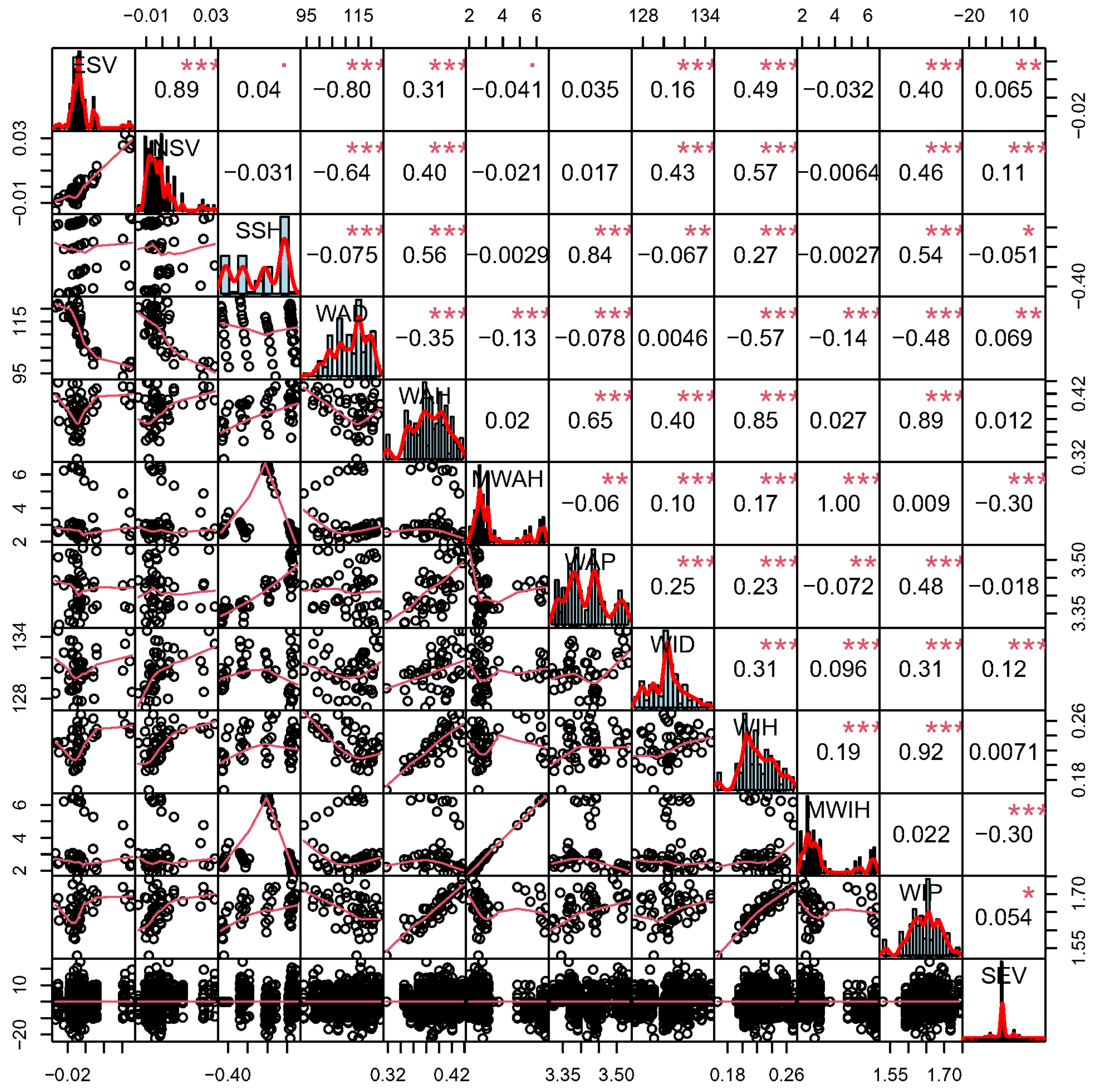
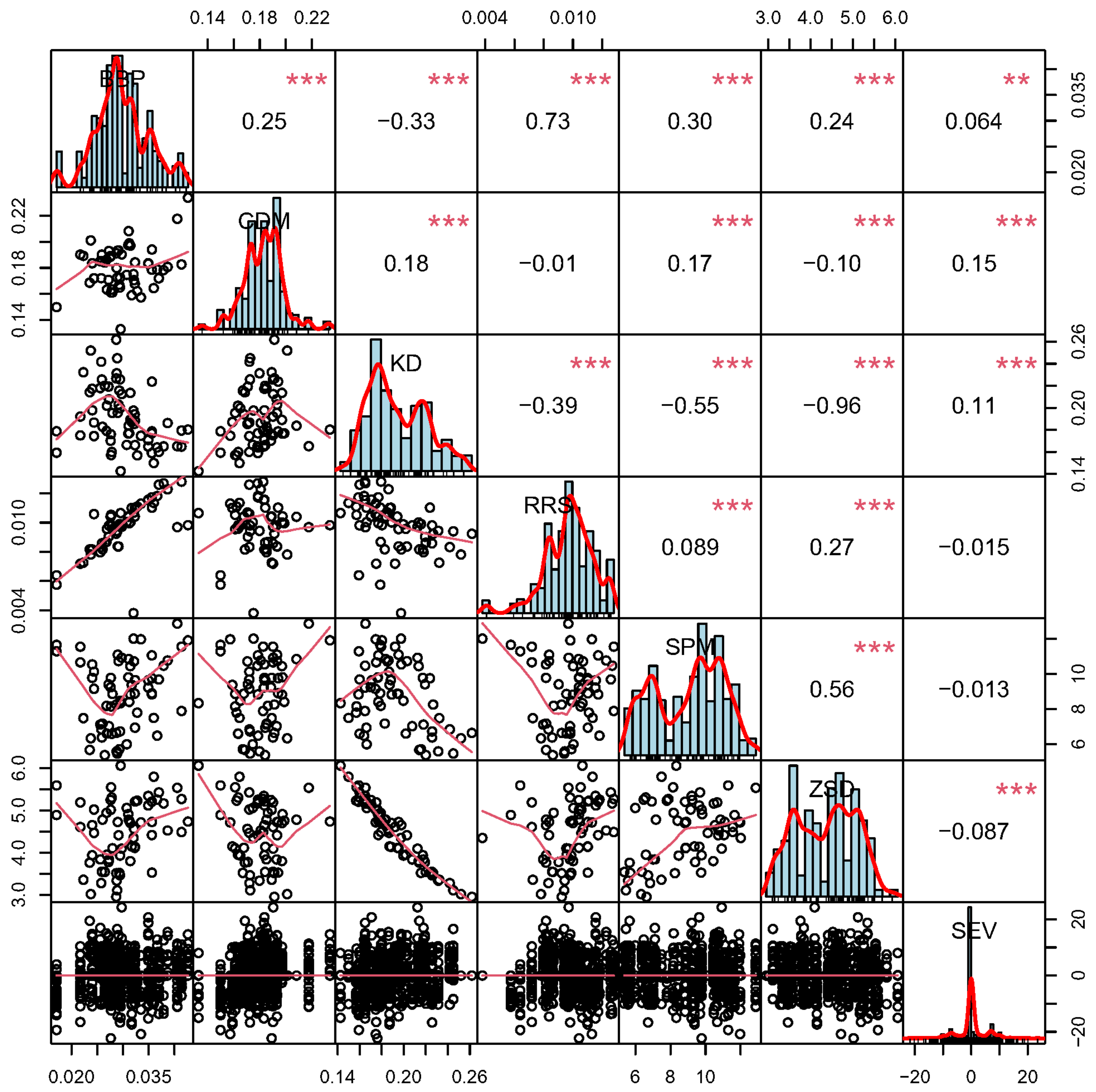
3.1. Correlation Analysis

As detailed in Section 2.3.2, the correlation analysis is aimed at (i) analyzing the interrelation among oceanographic, water quality, and shoreline evolution parameters; (ii) discarding high-correlated variables and, therefore, reducing the complexity of the designed BN model and computational time required for its implementation; and (iii) selecting the most relevant assessment endpoints to be included in the network.
Figure 3 and Figure 4 show the final output of the correlation analysis (i.e., the correlation matrix) implemented for the Adriatic coast of the lagoon of Venice for 16 variables reported in Table 1. In particular, Figure 3 focuses on the shoreline evolution trend and its physical oceanographic drivers, including winds, coastal currents, and sea level rises, whereas Figure 4 depicts the relation between shoreline evolution and water quality assessment endpoints.
In accordance with the study developed by [77] along the investigated coastal area, Figure 3 highlights how the evolution trend is mainly related to the maximum values of significant wave and wind wave height (30%). However, as in the case study of Venice, the difference between the two wave variables is negligible (>99%), and one can easily be excluded from the model design to be implemented as the second step in the multi-risk methodology (Figure 2). The same reason is also applied to the wind wave period, which is highly correlated to both significant wave and wind wave height (89% and 92%, respectively).
On the other hand, Figure 4 depicts the relation among the assessment endpoints, both shoreline evolution and water quality parameters. This second correlation analysis aims to avoid the redundancy of the assessment endpoints by selecting only three of them, including the shoreline evolution trend (SEV). Moreover, suspended particulate matter (SPM) represents the only chemical component of the turbidity of the water column, as it indicates the mass concentration of particulate (inorganic) matter in seawater. Therefore, the final step of this analysis consists of the identification of the physical element characterizing turbidity. Among them, diffuse attenuation (KD), which indicates the volume attenuation coefficient of downwelling radiative flux in seawater, is highly correlated to the other physical components, providing an overall good indicator of the process. At the same time, it shows one of the lowest correlation values with the other two selected assessment endpoints, hence achieving the object of this assessment.

3.2. Bayesian Network Model

After a short description of the main findings from the BN model design and parameterization, the calibration and validation of the model, and the sensitivity analysis, this section discusses the results of the BN application, including statistics, summarizing the probability distributions of the selected assessment endpoints under different ‘what if’ scenarios, representing extreme weather and oceanographic conditions for the reference period 2015–2019.

3.2.1. Model Design and Parametrization

The expert-based BN conceptual model aimed at assessing the coastal erosion risk and the related effects on water quality is depicted in Figure 5. The parent nodes of the model are oceanographic variables, including sea surface height (SSH), seawater velocity (i.e., NSV and ESV), and wind-wave parameters (i.e., WID, WIH, WAD, WAP, WAH, and MWAH). The selection of these variables was based on the literature review, expert opinions, and the above correlation analysis. For instance, wind and wave parameters (e.g., height, period, and direction), sea level, tide level, and water velocity were highlighted as the most influential factors to the shoreline changes [3,35,68,78]. Then, some of the variables were discarded to reduce the complexity of the BNs model such as the ones with a high correlation with other drives, as shown in Figure 3 and Figure 4 (e.g., MWIH vs. MWAH). On the other hand, the BN models’ child nodes are represented by the three assessment endpoints of the application (i.e., SEV, SPM, and KD), depicted in the lower part of Figure 5.
By using the discretize command in R, the input data for the baseline period (2015–2019) were discretized into a set of states to be integrated into the designed BN model. Based on the natural characteristics of each variable or node (e.g., continuous, Boolean values), the number of states was defined. Specifically, the oceanographic drivers were discretized into three equal-interval classes, whilst the assessment endpoint nodes (i.e., SEV, KD, and SPM) were manually classified into five classes to obtain a better visualization of results following the literature [68]. For example, SEV was discretized into five classes of “(−Inf, −10], (−10, −1], (−1,1], (1,12], (12, +Inf)”, where each class corresponds to “high erosion”, “moderate erosion”, “stable coast”, “moderate accretion”, and “high accretion”, respectively. Figure 5 shows the marginal distribution of all variables learned from the training data. A list of the final selected variables and their states is reported in Supplementary Materials Table S1.

3.2.2. Model Validation

The performance of the developed BN was evaluated by estimating the prediction error of the model, in terms of misclassification of unlabeled instances [79,80]. The results of the final BN model are depicted in Figure 6. Accordingly, the average predictive errors are 36.65%, 27.18%, and 27.53% for the SEV, SPM, and KD, respectively. This range of median classification errors is similar to the performance of some other BN applications, such as 34–45% for multi-sectoral flood damage assessment [81], 31–37% for freshwater ecosystem service assessment [31], about 29% for coastal vulnerability prediction [68], and 16–29% for estuarine ecosystem assessment [82]. Overall, the developed BN model could find the right estimation of about 63%, 72%, and 72% for the assessment endpoints; hence, the model allows one to have a good inference, as also verified by the outcomes of the validation process.

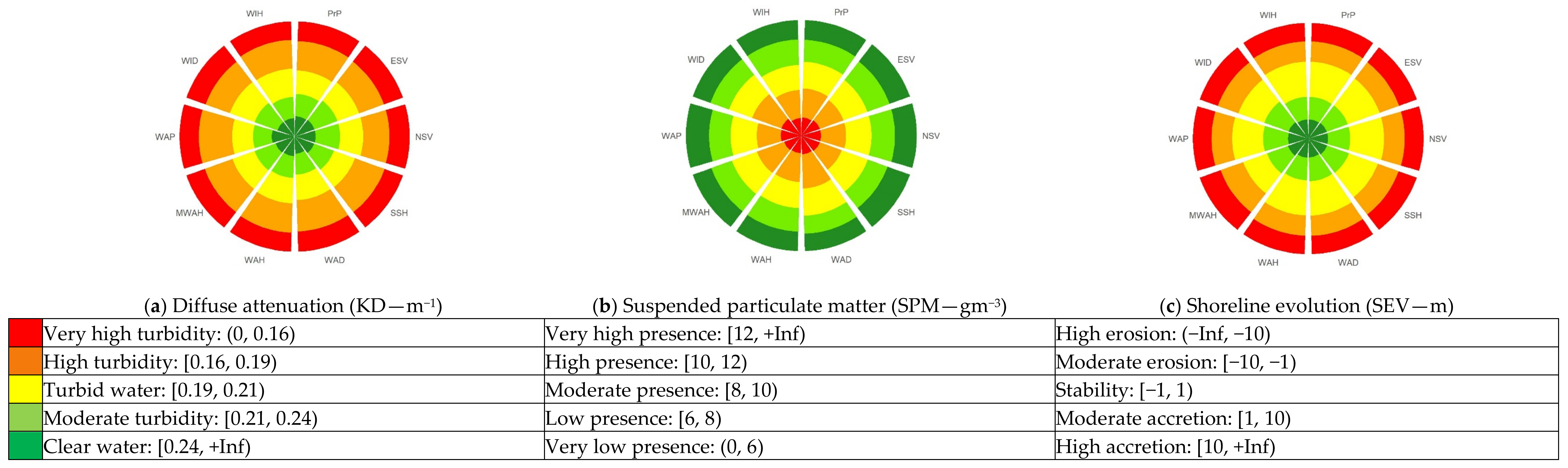
3.2.3. Sensitivity Analysis

Sensitivity analysis was performed to provide information on the sensitivity of the assessment endpoints (i.e., SEV, SPM, and KD) to changes in the explanatory variables and to identify the most influential variables on the BN model output. Therefore, analysis of each explanatory node was performed one by one, by setting the probability of its highest state to 100%, while all other nodes remained constant. Accordingly, the relative change in the posterior probability of each assessment endpoint was analyzed and compared among configurations by changing the probability of one variable at a time. Figure 7 shows the probability of the states of all assessment endpoints in comparison to the prior probability (PrP). Within the rose charts, the green segments represent the probability of classification in the states of low turbidity for KD and SPM, with high turbidity highlighted in the red segments. In the case of SEV, the green segments correspond to shoreline accretion, the yellow segments represent a stable shoreline, and the red represents an eroding shoreline. Compared to the prior probability, notable changes in the classification probabilities in SEV were seen from the changes in the maximum significant wind wave height, where the probability of the high-erosion classes increased, indicating the highest increase in shoreline variability. In comparison, SPM was more influenced by changes in wave direction and wind wave direction. High values of KD were generally most influenced by seawater velocity values (ESV and NSV); however, changes in the posterior probability to KD were more subtle, indicating that, overall, the explanatory nodes made roughly similar contributions to the model output.

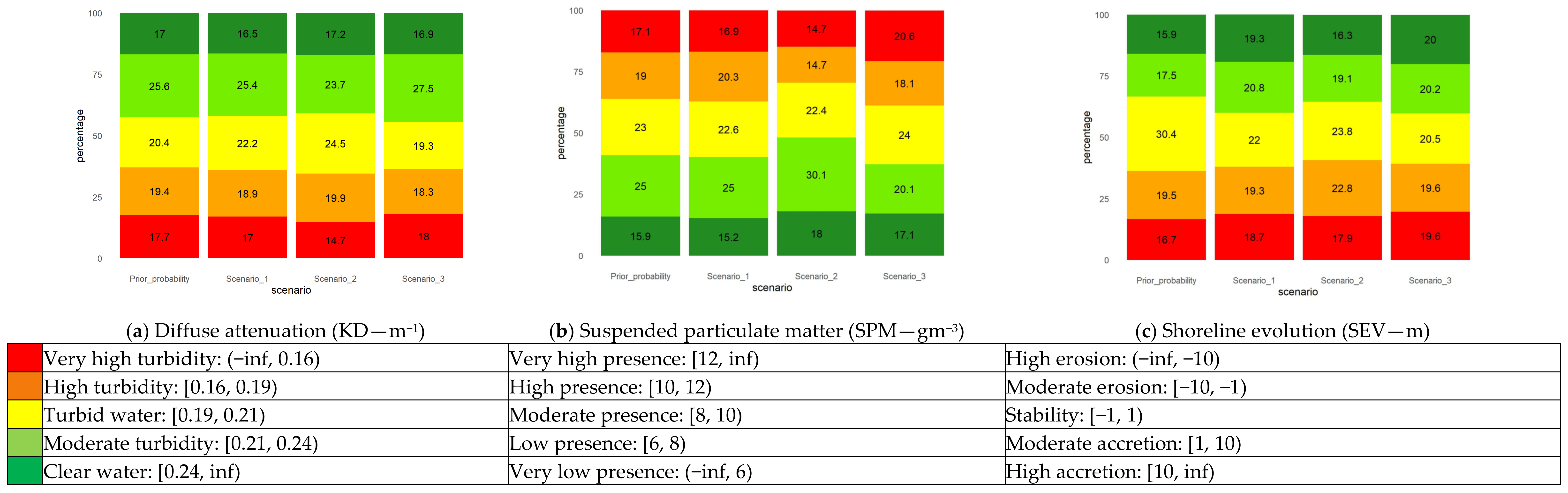
3.2.4. Baseline Scenario Analysis

Baseline scenario analysis was carried out by analyzing three different “what-if” scenarios representing extreme weather and oceanographic conditions for sea level rises, waves, wind wave height, and direction, as detailed in Section 2.3.3. Figure 8 shows the prior probability (i.e., the probability of the unperturbed condition to occur), depicted in the first bar of each assessment endpoint, as well as the results of three baseline scenarios in the second, third, and fourth bars, detailing the results of the first, second, and third scenarios.
First Scenario. The first ‘what-if’ scenario was set up by applying 100% probability of the highest state related to the maximum and mean significant wave height (i.e., MWAH and WAH, respectively). On the medium time scale (i.e., years to decades), the modifications in beach morphology and shoreline are affected by the changes in interannual wave-regime processes. Therefore, the prediction of future shoreline changes is often based on knowledge of the alongshore transport in relation to wave height [83]. The resulting shoreline evolution node highlights that the most significant change was observed in the [−1, 1] meters range, with a reduction of about 8.5% of stable coast (Figure 8). This change was balanced by an overall slight increase in the most unstable classes (i.e., high erosion (−Inf, −10) and high accretion [10, +Inf)). However, the variabilities were relatively lower (i.e., 3% and 2% rise in high-erosion and high-accretion class, respectively). There was about a 3% increase in the moderate-erosion class [−10, −1) and no change in moderate accretion [1, 10)). On the other hand, no significant changes were observed for the water quality assessment endpoint (i.e., about 1% for both KD and SPM), meaning that oceanographic pressures such as maximum and mean significant wave height could drive more severe impacts on the shoreline evolution rather than to water quality deterioration along the Venice shoreline.
The results of this scenario allow for evaluating the effect of wave height on shoreline dynamics and water quality parameters, as a prognostic inference. In fact, the increase in wave heights, resulting from changes in wind direction and surface wind energy [84], could contribute to the alteration in shoreline evolution since wave conditions are one of the main drivers of longshore drift rates [61] and longshore sediment transport rate [85]. Therefore, the alteration in maximum and mean significant wave height would have direct implications for coastal erosion, as observed in this scenario, i.e., reduce the stable class of shoreline evolution. As a consequence of longshore sediment transport, materials, organic and inorganic, can be carried away and redistributed by water and wind. Thus, the increase in wave height parameters could indirectly affect the deterioration of water quality parameters, such as KD and SPM. Nevertheless, this indirect influence was not clearly detected in this scenario analysis since the changes in these parameters were minor.
Second Scenario. The purpose of this scenario was to simulate wave and wind wave directions generated by the Sirocco wind along the Adriatic coastline, which has been identified as one of the main drivers of extreme storm surge events in the investigated area. Accordingly, the probabilities of the highest value of the wave and wind wave directions (i.e., WAD and WID) were set equal to [132, 135]° N and [114, 123]° N, respectively.
The results reported in Figure 8 for the shoreline evolution node show a very low increase in the upper and lower classes (i.e., high erosion and high accretion). Similar to the first scenario, the highest variability is observed once again in the stable class with a reduction of about 6.5%, which is compensated by an increase in the values of the two moderate classes (i.e., about 3% in moderate erosion and 1.5% in moderate accretion). On the other hand, as far as water quality variables are concerned, KD once again experienced no significant changes, while the SPM node showed a noticeable increase in both ‘high’ and ‘very high presence’ classes (about 6%). Therefore, the results show that both WAD and WID could influence water quality in terms of SPM, especially because of storm surge events driven by the Sirocco wind.
The results of this scenario help to disentangle the potential influence of wave and wind wave directions on shoreline dynamics and water quality parameters. An alteration in wind direction is recognized as the most important driver for sediment transport and coastal erosion [86,87,88]. Wind directions establish the wave direction and form seawater waves and wave height, which, in turn, disturb bottom sediment and affect shoreline dynamics. In the context of the Venice case study, the increase in extreme storm surge events, due to the changes in wind and wave direction, led to a reduction in the stable class because of the increased alteration in sediment transport, which, in turn, increased suspended particulate matter. The results of the scenario analysis also reflect that the mixing of sediment more significantly affects the presence of suspended particulate matter rather than the infiltration capacity of the light into the water since the changes in KD were negligible. It is important to highlight from the sensitivity analysis (Section 3.2.3) that wind direction is the most influential factor for the shoreline evolution (Figure 7c) and SPM (Figure 7b), which is in line with previous studies [61,89].
Third Scenario. The third scenario was aimed at evaluating the combination of the two most influencing extreme weather and oceanographic conditions affecting the investigated area, i.e., 100% probability of the highest classes of sea surface height (SSH) and maximum significant wave height (MWAH). As far as shoreline evolution is concerned, the results show that when storm waves reach critical height, small changes are observed in high- and moderate-erosion classes, with an increase of 3% and 4%, respectively. This result is balanced by a significant decrease of about 10% in the stable class, while the moderate and high accretion experienced slight changes (less than 2%). Regarding the water quality nodes, changes in SPM and KD are mostly countable (3% and 4%, respectively) for the highest and lowest classes, whereas moderate classes have almost negligible changes (less than 2%).
The results of this allow us to understand the effect of sea surface height and wave parameters on shoreline dynamics and water quality parameters. As emerged from many studies, sea level rise is expected to exacerbate beach erosion and long-term shoreline evolution [18,61,90,91]. The estimation of the sea level rise rate in Venice in 2100 is about 10.7 mm/year, with respect to the reference period (2000–2013) [92], and the future projections indicate that sea level rises could lead to the permanent loss of low-lying areas and beaches in this area [47]. Moreover, the increase in sea surface height is expected to reduce the effectiveness of the submerged and present coastal structures such as groins along the shore and jetties near the mouth. This scenario shows that the combined effect of SSH and MWAH could determine a reduction in the stable class of the shoreline up to 10%, which is higher than that obtained for scenario 1 (i.e., 6.5%) when considering only the changes in significant wave height.
The ‘what-if’ scenario analysis represents a first attempt to assess the impact of extreme weather and oceanographic condition impacts affecting the Adriatic coast of Venice. In particular, the overall baseline scenario analysis confirms that significant consequences could be related to coastal erosion risk and water quality changes under extreme sea level and wave conditions. This is in line with previous studies suggesting that changes in significant wave and wind wave height, as well as sea surface height, can perturb the coast and its dynamics, causing coastal erosion, flooding, increased turbidity, and other climate change-related impacts [45,91].

4. Conclusions

This work developed a risk assessment approach for the shoreline of Venice using a Bayesian Network model able to integrate different indicators representing drivers of shoreline evolution (waves, wind, extreme sea levels) and physical–chemical water quality parameters (diffuse attenuation and suspended particulate matter). The designed BN was validated by using the dataset for the period 2015–2019 in the case study area. After the correlation analysis and sensitivity analysis, three “what if” scenarios representing extreme weather and oceanographic events were simulated, testing the capability of the designed model to assess the potential consequences in terms of coastal erosion and water quality change. Accordingly, the designed BN model can be used as a decision support tool to support decision makers in the visualization of the potential risks of coastal erosion under a span of plausible extreme events.
The resulting outputs of this analysis, even to a minor extent, highlighted a relationship between alterations in oceanographic boundary conditions and coastal erosion and water quality parameters, with a rising probability of higher turbidity, as well as shoreline movement (i.e., accretion and retreat). Through the scenario analysis, changes in sea surface height, maximum, and mean significant wave height increased the probability of high-erosion and high-accretion states significantly compared to changes in the water quality variables (i.e., KD and SPM). However, by altering the wind and wave direction of currents, these WQ variables show significant changes in the higher-risk classes. These ‘what-if’ scenarios represent a first attempt at applying the BN model to assess the risks of climate change and variabilities of oceanic variables on coastal erosion and water quality parameters under different narrative scenarios. The results of this analysis present a clear relevance for coastal risk management in designing climate change impact assessments and local-level adaptation plans to cope with the impact of changing wind, wave, and current parameters in relation to climate change and sea level rises. Building on this model, future developments could be improved by including future climate change scenarios based on numerical modeling simulations.
The major advantages of the proposed Bayesian Network approach are the model transparency and flexibility (i.e., the connections among variables) and the possibility to incorporate both empirical data (e.g., satellite images and Marine Copernicus data) and expert knowledge (e.g., variable selection). Moreover, the BN model allows for the integration of heterogeneous data (i.e., wave data, water quality, and shoreline changes) from different sources with various spatio-temporal resolutions. Yet, the proposed BN demonstrates the flexibility in designing scenarios underpinning different hypotheses related to climate change projection and extreme events. Drawing from the results of this application, the model could be a useful tool for coastal managers and decision makers to assess the impacts of climate change and/or human interventions on shoreline changes and water quality-related problems, providing useful insights for coastal management.
Some constraints of the BN model are related to the data availability and spatio-temporal limitation. For instance, some relevant variables such as natural (e.g., precipitation) and anthropogenic variables (e.g., infrastructures and beach nourishment) were not considered in the model due to their incompleteness for the whole studied period. Moreover, the coarse spatial resolution (i.e., 4 km) of the oceanographic input data is a shortcoming of this analysis. Finally, the timeframe of this analysis remains short due to the availability of freely available satellite images for shoreline evolution analysis.
To overcome these limitations, future studies should expand the timeframe of the analysis by considering other sources of satellite images with higher temporal and spatial coverage such as the RapidEye Imagery. This expansion will allow for the integration of new variables such as sea level rise and storm surge dynamics, which could help the evaluation of the cascading impacts of extreme events against space and time dimensions. Moreover, the development of Dynamic Bayesian Networks could be implemented for the representation of the network’s dynamics among space and time. Finally, other novel methods, including more complex and advanced Machine Learning algorithms (e.g., Artificial Neural Network), could help to integrate more spatiotemporal data and simulate the complex dynamics and other natural processes arising in coastal areas.

Supplementary Materials

The following supporting information can be downloaded at: https://www.mdpi.com/article/10.3390/jmse12010139/s1, Table S1: List of the final selected variables and their states in BN model. Figure S1: Annual Net Shoreline Movement for the period 2015–2019.

Author Contributions

Conceptualization, H.V.P., M.K.D.B., E.F., S.T. and A.C.; methodology, H.V.P., M.K.D.B., M.P.S. and E.F.; software, H.V.P., M.K.D.B. and M.P.S.; validation, M.K.D.B. and M.P.S.; formal analysis, M.K.D.B. and M.P.S.; investigation, H.V.P., M.K.D.B. and E.F.; resources, H.V.P. and M.K.D.B.; data curation, H.V.P. and M.K.D.B.; writing—original draft preparation, H.V.P. and M.P.S.; writing—review and editing, M.K.D.B., E.F., S.T. and A.C.; visualization, H.V.P. and M.K.D.B.; supervision, E.F., S.T. and A.C.; project administration, S.T.; funding acquisition, S.T. All authors have read and agreed to the published version of the manuscript.

Funding

The research leading to these results was funded by the Venezia2021 project (http://www.corila.it/it/Venezia2021, 20 November 2023). Scientific activities were performed with the contribution of the Provveditorato for the Public Works of Veneto, Trentino Alto Adige, and Friuli Venezia Giulia, provided through the concessionary of State Consorzio Venezia Nuova and coordinated by CORILA. The work was also funded by the SAVEMEDCOASTS-2 project (https://www.savemedcoasts2.eu/).

Institutional Review Board Statement

Not applicable.

Informed Consent Statement

Not applicable.

Data Availability Statement

Data sources are detailed in Table 1.

Conflicts of Interest

The authors declare no conflicts of interest.

References

  1. IPCC. Chapter 6: Coastal Zones and Marine Ecosystems. In Climate Change 2001: Impacts, Adaptation and Vulnerability; IPCC: Geneva, Switzerland, 2003; pp. 345–379. Available online: https://www.grida.no/publications/269 (accessed on 17 December 2022).
  2. IPCC. Climate Change 2014 Synthesis Report. Contribution of Working Groups I, II and III to the Fifth Assessment Report of the Intergovernmental Panel on Climate Change; IPCC: Geneva, Switzerland, 2014; pp. 1–112. [Google Scholar]
  3. Poelhekke, L.; Jäger, W.S.; van Dongeren, A.; Plomaritis, T.A.; McCall, R.; Ferreira, Ó. Predicting coastal hazards for sandy coasts with a Bayesian Network. Coast. Eng. 2016, 118, 21–34. [Google Scholar] [CrossRef]
  4. Estrela-Segrelles, C.; Gómez-Martinez, G.; Pérez-Martín, M.Á. Risk assessment of climate change impacts on Mediterranean coastal wetlands. Application in Júcar River Basin District (Spain). Sci. Total Environ. 2021, 790, 148032. [Google Scholar] [CrossRef] [PubMed]
  5. Bastidas-Arteaga, E.; Creach, A. Climate change for coastal areas: Risks, adaptation and acceptability. Adv. Clim. Chang. Res. 2020, 11, 295–296. [Google Scholar] [CrossRef]
  6. Hoegh-Guldberg, O.; Bruno, J. The impact of climate change on the world’s marine ecosystems. Science 2010, 328, 1523–1528. [Google Scholar] [CrossRef]
  7. Halpern, B.S.; Lbridge, S.; Selkoe, K.A.; Kappel, C.V.; Micheli, F.; D’Agrosa, C.; Bruno, J.F.; Casey, K.S.; Ebert, C.; Fox, H.E.; et al. A global map of human impact on marine ecosystems. Science 2008, 319, 948–952. [Google Scholar] [CrossRef] [PubMed]
  8. Halpern, B.S.; Frazier, M.; Afflerbach, J.; Lowndes, J.S.; Micheli, F.; O’Hara, C.; Scarborough, C.; Selkoe, K.A. Recent pace of change in human impact on the world’s ocean. Sci. Rep. 2019, 9, 11609. [Google Scholar] [CrossRef]
  9. IPCC. Summary for Policymakers. In Climate Change 2014: Impacts, Adaptation, and Vulnerability; Field, C.B., Barros, V.R., Dokken, D.J., Mach, K.J., Mastrandrea, M.D., Bilir, T.E., Chatterjee, M., Ebi, K.L., Estrada, Y.O., Genova, R.C., et al., Eds.; Cambridge University Press: Cambridge, UK; New York, NY, USA, 2014. [Google Scholar]
  10. Ferrarin, C.; Valentini, A.; Vodopivec, M.; Klaric, D.; Massaro, G.; Bajo, M.; Carraro, E. Integrated sea storm management strategy: The 29 October 2018 event in the Adriatic Sea. Nat. Hazards Earth Syst. Sci. 2020, 20, 73–93. [Google Scholar] [CrossRef]
  11. Fontolan, G.; Bezzi, A.; Martinucci, D.; Pillon, S.; Popesso, C.; Rizzetto, F. Sediment budget and management of the Veneto beaches, Italy: An application of the Littoral Cells Management System (SICELL). In Proceedings of the Conférence Méditerranéenne Côtière et Maritime, Ferrara, Italy, 25–27 November 2015; pp. 47–50. [Google Scholar] [CrossRef]
  12. Morucci, S.; Coraci, E.; Crosato, F.; Ferla, M. Extreme events in Venice and in the North Adriatic Sea: 28–29 October 2018. Sci. Fis. Nat. 2020, 31, 113–122. [Google Scholar] [CrossRef]
  13. Tosi, L.; Da Lio, C.; Donnici, S.; Strozzi, T.; Teatini, P. Vulnerability of Venice’s coastland to relative sea-level rise. Proc. Int. Assoc. Hydrol. Sci. 2020, 382, 689–695. [Google Scholar] [CrossRef]
  14. Van Rijn, L.C. Coastal erosion and control. Ocean Coast. Manag. 2011, 54, 867–887. [Google Scholar] [CrossRef]
  15. Quartel, S.; Kroon, A.; Ruessink, B.G. Seasonal accretion and erosion patterns of a microtidal sandy beach. Mar. Geol. 2008, 250, 19–33. [Google Scholar] [CrossRef]
  16. Mentaschi, L.; Vousdoukas, M.I.; Pekel, J.F.; Voukouvalas, E.; Feyen, L. Global long-term observations of coastal erosion and accretion. Sci. Rep. 2018, 8, 12876. [Google Scholar] [CrossRef] [PubMed]
  17. Thorne, C.R.; Evans, E.P.; Penning-rowsell, E.C. Future Flooding and Coastal Erosion Risks; Thomas Telford Publishing: London, UK, 2007. [Google Scholar] [CrossRef]
  18. Vecchio, A.; Anzidei, M.; Serpelloni, E. Sea level rise projections up to 2150 in the northern Mediterranean coasts. Environ. Res. Lett. 2024, 19, 014050. [Google Scholar] [CrossRef]
  19. Oppenheimer. The irreversible momentum of clean energy: Private-sector efforts help drive decoupling of emissions and economic growth. Science 2017, 355, 126–129. [Google Scholar] [CrossRef] [PubMed]
  20. PNACC. Piano Nazionale di Adattamento ai Cambiamenti Climatici PNACC. 2017. Available online: https://politichecoesione.governo.it/media/2868/pnacc_luglio-2017.pdf (accessed on 17 December 2022).
  21. Loizidou, X.I.; Orthodoxou, D.L.; Loizides, M.I.; Petsa, D.; Anzidei, M. Adapting to sea level rise: Participatory, solution-oriented policy tools in vulnerable Mediterranean areas. Environ. Syst. Decis. 2023. [Google Scholar] [CrossRef] [PubMed]
  22. Prasad, D.H.; Kumar, N.D. Coastal Erosion Studies—A Review. Int. J. Geosci. 2014, 5, 341–345. [Google Scholar] [CrossRef]
  23. Erdem, F.; Bayram, B.; Bakirman, T.; Bayrak, O.C.; Akpinar, B. An ensemble deep learning based shoreline segmentation approach (WaterNet) from Landsat 8 OLI images. Adv. Sp. Res. 2021, 67, 964–974. [Google Scholar] [CrossRef]
  24. Toure, S.; Diop, O.; Kpalma, K.; Maiga, A.S. Shoreline detection using optical remote sensing: A review. ISPRS Int. J. Geo-Inf. 2019, 8, 75. [Google Scholar] [CrossRef]
  25. Vos, K.; Splinter, K.D.; Harley, M.D.; Simmons, J.A.; Turner, I.L. CoastSat: A Google Earth Engine-enabled Python toolkit to extract shorelines from publicly available satellite imagery. Environ. Model. Softw. 2019, 122, 104528. [Google Scholar] [CrossRef]
  26. Vitousek, S.; Vos, K.; Splinter, K.D.; Erikson, L.; Barnard, P.L. A Model Integrating Satellite-Derived Shoreline Observations for Predicting Fine-Scale Shoreline Response to Waves and Sea-Level Rise Across Large Coastal Regions. J. Geophys. Res. Earth Surf. 2023, 128, e2022JF006936. [Google Scholar] [CrossRef]
  27. Castelle, B.; Masselink, G.; Scott, T.; Stokes, C.; Konstantinou, A.; Marieu, V.; Bujan, S. Satellite-derived shoreline detection at a high-energy meso-macrotidal beach. Geomorphology 2021, 383, 107707. [Google Scholar] [CrossRef]
  28. El-Asmar, H.M.; Hereher, M.E.; El Kafrawy, S.B. Surface area change detection of the Burullus Lagoon, North of the Nile Delta, Egypt, using water indices: A remote sensing approach. Egypt. J. Remote Sens. Sp. Sci. 2013, 16, 119–123. [Google Scholar] [CrossRef]
  29. Zennaro, F.; Furlan, E.; Simeoni, C.; Torresan, S.; Aslan, S.; Critto, A.; Marcomini, A. Exploring machine learning potential for climate change risk assessment. Earth-Sci. Rev. 2021, 220, 103752. [Google Scholar] [CrossRef]
  30. Furlan, E.; Slanzi, D.; Torresan, S.; Critto, A.; Marcomini, A. Multi-scenario analysis in the Adriatic Sea: A GIS-based Bayesian network to support maritime spatial planning. Sci. Total Environ. 2020, 703, 134972. [Google Scholar] [CrossRef] [PubMed]
  31. Pham, H.V.; Sperotto, A.; Torresan, S.; Critto, A.; Marcomini, A. Integrating Bayesian Networks into ecosystem services assessment to support water management at the river basin scale. Ecosyst. Serv. 2021, 50, 101300. [Google Scholar] [CrossRef]
  32. Sperotto, A.; Molina, J.-L.; Torresan, S.; Critto, A.; Marcomini, A. Reviewing Bayesian Networks potentials for climate change impacts assessment and management: A multi-risk perspective. J. Environ. Manag. 2017, 202, 320–331. [Google Scholar] [CrossRef]
  33. Moe, S.J.; Carriger, J.F.; Glendell, M. Increased Use of Bayesian Network Models Has Improved Environmental Risk Assessments. Integr. Environ. Assess. Manag. 2021, 17, 53–61. [Google Scholar] [CrossRef] [PubMed]
  34. Kaikkonen, L.; Parviainen, T.; Rahikainen, M.; Uusitalo, L.; Lehikoinen, A. Bayesian Networks in Environmental Risk Assessment: A Review. Integr. Environ. Assess. Manag. 2021, 17, 62–78. [Google Scholar] [CrossRef]
  35. Jäger, W.S.; Christie, E.K.; Hanea, A.M.; den Heijer, C.; Spencer, T. A Bayesian network approach for coastal risk analysis and decision making. Coast. Eng. 2018, 134, 48–61. [Google Scholar] [CrossRef]
  36. Sahin, O.; Stewart, R.A.; Faivre, G.; Ware, D.; Tomlinson, R.; Mackey, B. Spatial Bayesian Network for predicting sea level rise induced coastal erosion in a small Pacific Island. J. Environ. Manag. 2019, 238, 341–351. [Google Scholar] [CrossRef]
  37. Bezzi, A.; Fontolan, G.; Nordstrom, K.F.; Carrer, D.; Jackson, N.L. Beach Nourishment and Foredune Restoration: Practices and Constraints along the Venetian Shoreline, Italy. J. Coast. Res. 2009, 1, 287–291. [Google Scholar]
  38. Rizzi, J.; Torresan, S.; Zabeo, A.; Critto, A.; Tosoni, A.; Tomasin, A.; Marcomini, A. Assessing storm surge risk under future sea-level rise scenarios: A case study in the North Adriatic coast. J. Coast. Conserv. 2017, 21, 453–471. [Google Scholar] [CrossRef]
  39. Zoccarato, C.; Da Lio, C. The Holocene influence on the future evolution of the Venice Lagoon tidal marshes. Commun. Earth Environ. 2021, 2, 77. [Google Scholar] [CrossRef]
  40. Pham, H.V.; Dal Barco, M.K.; Cadau, M.; Harris, R.; Furlan, E.; Torresan, S.; Rubinetti, S.; Zanchettin, D.; Rubino, A.; Kuznetsov, I.; et al. Multi-model chain for climate change scenario analysis to support coastal erosion and water quality risk management for the Metropolitan city of Venice. Sci. Total Environ. 2023, 904, 166310. [Google Scholar] [CrossRef] [PubMed]
  41. Alberti, T.; Anzidei, M.; Faranda, D.; Vecchio, A.; Favaro, M.; Papa, A. Dynamical diagnostic of extreme events in Venice lagoon and their mitigation with the MoSE. Sci. Rep. 2023, 13, 10475. [Google Scholar] [CrossRef]
  42. Faranda, D.; Ginesta, M.; Alberti, T.; Coppola, E.; Anzidei, M. Attributing Venice Acqua Alta events to a changing climate and evaluating the efficacy of MoSE adaptation strategy. npj Clim. Atmos. Sci. 2023, 6, 181. [Google Scholar] [CrossRef]
  43. Solidoro, C.; Bandelj, V.; Bernardi, F.A.; Camatti, E.; Ciavatta, S.; Cossarini, G.; Facca, C.; Franzoi, P.; Libralato, S.; Canu, D.M.; et al. Response of the Venice Lagoon ecosystem to natural and anthropogenic pressures over the last 50 years. In Coastal Lagoons; Critical Habitats of Environmental Change; CRC Press: Boca Raton, FL, USA, 2010; pp. 483–511. [Google Scholar] [CrossRef]
  44. Fogarin, S.; Madricardo, F.; Zaggia, L.; Sigovini, M.; Montereale-Gavazzi, G.; Kruss, A.; Lorenzetti, G.; Manfé, G.; Petrizzo, A.; Molinaroli, E.; et al. Tidal inlets in the Anthropocene: Geomorphology and benthic habitats of the Chioggia inlet, Venice Lagoon (Italy). Earth Surf. Process. Landf. 2019, 44, 2297–2315. [Google Scholar] [CrossRef]
  45. Lionello, P.; Barriopedro, D.; Ferrarin, C.; Nicholls, R.J.; Orlic, M.; Reale, M.; Umgiesser, G.; Vousdoukas, M.; Zanchettin, D. Extremes floods of Venice: Characteristics, dynamics, past and future evolution. Nat. Hazards Earth Syst. Sci. 2020, 21, 2705–2731. [Google Scholar] [CrossRef]
  46. Zanchettin, D.; Bruni, S.; Raicich, F.; Lionello, P.; Adloff, F.; Androsov, A.; Antonioli, F.; Artale, V.; Carminati, E.; Ferrarin, C.; et al. Review article: Sea-level rise in Venice: Historic and future trends. Nat. Hazards Earth Syst. Sci. Discuss. 2020, 21, 2643–2678. [Google Scholar] [CrossRef]
  47. Vecchio, A.; Anzidei, M.; Serpelloni, E.; Florindo, F. Natural variability and vertical land motion contributions in the Mediterranean sea-level records over the last two centuries and projections for 2100. Water 2019, 11, 1480. [Google Scholar] [CrossRef]
  48. Pomaro, A.; Cavaleri, L.; Lionello, P. Climatology and trends of the Adriatic Sea wind waves: Analysis of a 37-year long instrumental data set. Int. J. Climatol. 2017, 37, 4237–4250. [Google Scholar] [CrossRef]
  49. Da Lio, C.; Tosi, L. Vulnerability to relative sea-level rise in the Po river delta (Italy). Estuar. Coast. Shelf Sci. 2019, 228, 106379. [Google Scholar] [CrossRef]
  50. Tosi, L.; Da Lio, C.; Strozzi, T.; Teatini, P. Combining L- and X-Band SAR interferometry to assess ground displacements in heterogeneous coastal environments: The Po River Delta and Venice Lagoon, Italy. Remote Sens. 2016, 8, 308. [Google Scholar] [CrossRef]
  51. Carbognin, L.; Teatini, P.; Tosi, L.; Strozzi, T.; Tomasin, A. Present Relative Sea Level Rise in the Northern Adriatic Coastal Area. Coast. Mar. Spat. Plan. 2010, 1147–1162. Available online: https://core.ac.uk/download/pdf/33155996.pdf (accessed on 20 November 2023).
  52. Scardino, G.; Anzidei, M.; Petio, P.; Serpelloni, E.; De Santis, V.; Rizzo, A.; Liso, S.I.; Zingaro, M.; Capolongo, D.; Vecchio, A.; et al. The Impact of Future Sea-Level Rise on Low-Lying Subsiding Coasts: A Case Study of Tavoliere Delle Puglie (Southern Italy). Remote Sens. 2022, 14, 4936. [Google Scholar] [CrossRef]
  53. Molinaroli, E.; Guerzoni, S.; Suman, D. Do the Adaptations of Venice and Miami to Sea Level Rise Offer Lessons for Other Vulnerable Coastal Cities? Environ. Manag. 2019, 64, 391–415. [Google Scholar] [CrossRef]
  54. Ramieri, E.; Hartley, A.; Office, M.; Barbanti, A.; National, I.; Santos, F.D. Methods for Assessing Coastal Vulnerability to Climate Change; ETC CCA Technical Paper 1/2011; ETC/CCA: Bologna, Italy, 2011. [Google Scholar] [CrossRef]
  55. Ruol, P.; Martinelli, L.; Favaretto, C.; Pinato, T.; Galiazzo, F.; Patti, S.; Anti, U.; Piazza, R.; Simonin, P.; Selvi, G. Gestione Integrata Della Zona Costiera Studio E Monitoraggio Per La Definizione Degli Interventi Di Difesa Dei Litorali Dall’erosione Nella Regione Veneto-Linee Guida; Edizioni Progetto Padova: Padova, Italy, 2016. [Google Scholar]
  56. Facca, C.; Bonometto, A.; Boscolo, R.; Buosi, A.; Parravicini, M.; Siega, A.; Volpe, V.; Sfriso, A. Coastal lagoon recovery by seagrass restoration. A new strategic approach to meet HD & WFD objectives. In Proceedings of the 9th European Conference on Ecological Restoration, Oulu, Finland, 3–8 August 2014; pp. 3–8. [Google Scholar]
  57. European Commission. EU Climate Adaptation Strategy. 2021. Available online: https://eur-lex.europa.eu/legal-content/EN/TXT/PDF/?uri=CELEX:52021DC0082&from=EN (accessed on 20 November 2023).
  58. Scutari, M. Learning Bayesian Networks with the bnlearn R package. J. Stat. Softw. 2010, 35, 1–22. [Google Scholar] [CrossRef]
  59. Fogarin, S.; Zanetti, M.; Dal Barco, M.K.; Zennaro, F.; Furlan, E.; Torresan, S.; Pham, H.V.; Critto, A. Combining remote sensing analysis with machine learning to evaluate short-term coastal evolution trend in the shoreline of Venice. Sci. Total Environ. 2023, 859, 160293. [Google Scholar] [CrossRef]
  60. Chataigner, T.; Yates, M.L.; Le Dantec, N.; Harley, M.D.; Splinter, K.D.; Goutal, N. Sensitivity of a one-line longshore shoreline change model to the mean wave direction. Coast. Eng. 2022, 172, 104025. [Google Scholar] [CrossRef]
  61. Zacharioudaki, A.; Reeve, D.E. Shoreline evolution under climate change wave scenarios. Clim. Chang. 2011, 108, 73–105. [Google Scholar] [CrossRef]
  62. Wright, R.E. Logistic regression. In Reading and Understanding Multivariate Statistics; American Psychological Association: Washington, DC, USA, 1995. [Google Scholar]
  63. Graupe, D. Principles of Artificial Neural Networks; World Scientific: Singapore, 2013; Volume 7, ISBN 9814522759. [Google Scholar]
  64. Breiman, L.E.O. Random Forests. Mach. Learn. 2001, 45, 5–32. [Google Scholar] [CrossRef]
  65. UNDP. Egypt’s National Strategy for Adaptation to Climate Change and Disaster Risk Reduction; Food and Agriculture Organization: Rome, Italy, 2011. [Google Scholar]
  66. IPCC. Climate Change 2014: Impacts, Adaptation, and Vulnerability. Part B: Regional Aspects. Contribution of Working Group II to the Fifth Assessment Report of the Intergovernmental Panel on Climate Change; Cambridge University Press: Cambridge, UK, 2014; p. 688. [Google Scholar] [CrossRef]
  67. Schulzweida, U. Climate Data Operator (CDO) User Guide (Version 1.9.5). no. August, pp. 1–217. 2018. Available online: https://code.mpimet.mpg.de/projects/cdo/embedded/cdo.pdf (accessed on 17 December 2022).
  68. Gutierrez, B.T.; Plant, N.G.; Thieler, E.R. A Bayesian network to predict coastal vulnerability to sea level rise. J. Geophys. Res. Earth Surf. 2011, 116, 1–15. [Google Scholar] [CrossRef]
  69. Scutari, M. Bayesian network constraint-based structure learning algorithms: Parallel and optimized implementations in the bnlearn R package. J. Stat. Softw. 2017, 77, 1–20. [Google Scholar] [CrossRef]
  70. Kragt, M.E. A Beginners Guide to Bayesian Network Modelling for Integrated Catchment. 2009. Available online: www.landscapelogic.org.au (accessed on 17 December 2022).
  71. Pollino, C.A.; Woodberry, O.; Nicholson, A.; Korb, K.; Hart, B.T. Parameterisation and evaluation of a Bayesian network for use in an ecological risk assessment. Environ. Model. Softw. 2007, 22, 1140–1152. [Google Scholar] [CrossRef]
  72. Stelzenmüller, V.; Lee, J.; Garnacho, E.; Rogers, S.I. Assessment of a Bayesian Belief Network–GIS framework as a practical tool to support marine planning. Mar. Pollut. Bull. 2010, 60, 1743–1754. [Google Scholar] [CrossRef]
  73. Coupé, V.M.H.; Peek, N.; Ottenkamp, J.; Habbema, J.D.F. Using sensitivity analysis for efficient quantification of a belief network. Artif. Intell. Med. 1999, 17, 223–247. [Google Scholar] [CrossRef] [PubMed]
  74. Gačić, M.; Kovačević, V.; Cosoli, S.; Mazzoldi, A.; Paduan, J.D.; Mancero-Mosquera, I.; Yari, S. Surface current patterns in front of the Venice Lagoon. Estuar. Coast. Shelf Sci. 2009, 82, 485–494. [Google Scholar] [CrossRef]
  75. Benetazzo, A.; Fedele, F.; Carniel, S.; Ricchi, A.; Bucchignani, E.; Sclavo, M. Wave climate of the Adriatic Sea: A future scenario simulation. Nat. Hazards Earth Syst. Sci. 2012, 12, 2065–2076. [Google Scholar] [CrossRef]
  76. Benetazzo, A.; Carniel, S.; Sclavo, M.; Bergamasco, A. Wave–current interaction: Effect on the wave field in a semi-enclosed basin. Ocean Model. 2013, 70, 152–165. [Google Scholar] [CrossRef]
  77. Ruol, P.; Martinelli, L.; Favaretto, C. Vulnerability analysis of the Venetian littoral and adopted mitigation strategy. Water 2018, 10, 984. [Google Scholar] [CrossRef]
  78. Plomaritis, T.A.; Costas, S.; Ferreira, Ó. Use of a Bayesian Network for coastal hazards, impact and disaster risk reduction assessment at a coastal barrier (Ria Formosa, Portugal). Coast. Eng. 2018, 134, 134–147. [Google Scholar] [CrossRef]
  79. Rodrìguez, J.D.; Aritz Pérez, A.; Lozano, J.A. Sensitivity Analysis of k-Fold Cross Validation in Prediction Error Estimation. IEEE Trans. Pattern Anal. Mach. Intell. 2010, 32, 569–575. [Google Scholar] [CrossRef]
  80. Stone, M. Cross validatory choice and assessment of statistical predictions. J. R. Stat. Soc. Ser. B 1974, 36, 111–133. [Google Scholar] [CrossRef]
  81. Harris, R.; Furlan, E.; Pham, H.V.; Torresan, S.; Mysiak, J.; Critto, A. A Bayesian network approach for multi-sectoral flood damage assessment and multi-scenario analysis. Clim. Risk Manag. 2022, 35, 100410. [Google Scholar] [CrossRef]
  82. Bulmer, R.H.; Stephenson, F.; Lohrer, A.M.; Lundquist, C.J.; Madarasz-Smith, A.; Pilditch, C.A.; Thrush, S.F.; Hewitt, J.E. Informing the management of multiple stressors on estuarine ecosystems using an expert-based Bayesian Network model. J. Environ. Manag. 2022, 301, 113576. [Google Scholar] [CrossRef]
  83. Coelho, C.; Silva, R.; Veloso-Gomes, F.; Taveira-Pinto, F. Potential effects of climate change on northwest portuguese coastal zones. ICES J. Mar. Sci. 2009, 66, 1497–1507. [Google Scholar] [CrossRef]
  84. Franco-Ochoa, C.; Zambrano-Medina, Y.; Plata-Rocha, W.; Monjardín-Armenta, S.; Rodríguez-Cueto, Y.; Escudero, M.; Mendoza, E. Long-term analysis of wave climate and shoreline change along the gulf of California. Appl. Sci. 2020, 10, 8719. [Google Scholar] [CrossRef]
  85. Tomasicchio, G.R.; Francone, A.; Simmonds, D.J.; D’Alessandro, F.; Frega, F. Prediction of shoreline evolution. Reliability of a general model for the mixed beach case. J. Mar. Sci. Eng. 2020, 8, 361. [Google Scholar] [CrossRef]
  86. Kondrat, V.; Šakurova, I.; Baltranaitė, E.; Kelpšaitė-Rimkienė, L. Natural and anthropogenic factors shaping the shoreline of klaipėda, Lithuania. J. Mar. Sci. Eng. 2021, 9, 1456. [Google Scholar] [CrossRef]
  87. Kelpšaite, L.; Dailidiene, I. Influence of wind wave climate change on coastal processes in the eastern Baltic Sea. J. Coast. Res. 2011, 2011, 220–224. [Google Scholar]
  88. Susanti, I.; Nurlatifah, A.; Martono; Maryadi, E.; Slamet, S.L.; Siswanto, B.; Suhermat, M. Abrasion and accretion dynamics as impact of climate change in coastal area of Yogyakarta. AIP Conf. Proc. 2021, 2331, 030009. [Google Scholar] [CrossRef]
  89. Dickson, M.E.; Walkden, M.J.A.; Hall, J.W. Systemic impacts of climate change on an eroding coastal region over the twenty-first century. Clim. Chang. 2007, 84, 141–166. [Google Scholar] [CrossRef]
  90. Leatherman, S.P.; Zhang, K.; Douglas, B.C. Sea level rise shown to drive coastal erosion. Eos 2000, 81, 55–57. [Google Scholar] [CrossRef]
  91. Scardino, G.; Sabatier, F.; Scicchitano, G.; Piscitelli, A.; Milella, M.; Vecchio, A.; Anzidei, M.; Mastronuzzi, G. Sea-level rise and shoreline changes along an open sandy coast: Case study of gulf of taranto, Italy. Water 2020, 12, 1414. [Google Scholar] [CrossRef]
  92. Antonioli, F.; Anzidei, M.; Amorosi, A.; Lo Presti, V.; Mastronuzzi, G.; Deiana, G.; De Falco, G.; Fontana, A.; Fontolan, G.; Lisco, S.; et al. Sea-level rise and potential drowning of the Italian coastal plains: Flooding risk scenarios for 2100. Quat. Sci. Rev. 2017, 158, 29–43. [Google Scholar] [CrossRef]
Figure 1. The Metropolitan City of Venice littoral, including Pellestrina, Lido, and Cavallino. The length of the transects was increased for better visualization.
Jmse 12 00139 g001
Figure 2. Bayesian Network model for the risk assessment related to coastal erosion and water quality. Abbreviation: SEV—shoreline evolution; WQ—water quality; CMEMS—Copernicus Marine Service.
Jmse 12 00139 g002
Figure 3. Correlation matrix focusing on the relation between shoreline evolution and oceanographic variables. The distribution of each variable is shown on the diagonal. Below the diagonal: the bivariate scatter plots with a fitted line are displayed. Above the diagonal: the value of the correlation and the significance level as stars: p-values (0, 0.001, 0.01, 0.05, 0.1, 1) and equivalent symbols (“***”, “**”, “*”, “.”, “ ”).
Jmse 12 00139 g003
Figure 4. Correlation matrix focusing on shoreline evolution and water quality variables. The distribution of each variable is shown on the diagonal. Below the diagonal: the bivariate scatter plots with a fitted line are displayed. Above the diagonal: the value of the correlation and the significance level as stars: p-values (0, 0.001, 0.01, 0.05, 0.1, 1) and equivalent symbols (“***”, “**”, “*”, “.”, “ ”).
Jmse 12 00139 g004
Figure 5. Final BN model reporting the marginal distributions in the study period (2015–2019) associated to all variables included in the network.
Jmse 12 00139 g005
Figure 6. BN model validation, Boxplot that reports the average BN-model losses in terms of classification errors of assessment endpoints (i.e., shoreline evolution (SEV), suspended matter (SPM), and diffuse attenuation (KD)).
Jmse 12 00139 g006
Figure 7. Sensitivity analysis for the explanatory nodes of the constructed BN model for the assessment endpoints. The red, yellow and dark green sections represent the highest, moderate, and lowest classes, respectively.
Jmse 12 00139 g007
Figure 8. Results of diagnostic inference of the three baseline scenarios for the three selected assessment endpoints. The red, yellow, and green colors represent the different classes of each variable, as detailed in the box.
Jmse 12 00139 g008
Table 1. Available dataset for the implementation of the coastal erosion risk assessment methodology in the Venice case study.
VariableAbbreviationUnitSpatial DomainSpatial
Resolution
Timeframe
Available
Data
Format
Reference/Link
Sea surface height above the geoidSSHmMediterranean Sea0.0625 degrees1987–2023NetCDFhttps://doi.org/10.25423/CMCC/MEDSEA_MULTIYEAR_PHY_006_004_E3R1 (accessed on 19 August 2022)
Eastward sea water velocityESVm s−1Mediterranean Sea0.0625 degrees1987–2023NetCDF
Northward sea water velocityNSVm s−1Mediterranean Sea0.0625 degrees1987–2023NetCDF
Wave direction fromWADdegreeMediterranean Sea0.042 degrees1993–2023NetCDFhttps://doi.org/10.25423/cmcc/medsea_multiyear_wav_006_012 (accessed on 19 August 2022)
Significant wave heightWAHmMediterranean Sea0.042 degrees1993–2023NetCDF
Sea surface wave mean periodWAPsMediterranean Sea0.042 degrees1993–2023NetCDF
Wind wave directionWIDdegreeMediterranean Sea0.042 degrees1993–2023NetCDF
Significant wind wave heightWIHmMediterranean Sea0.042 degrees1993–2023NetCDF
Sea-surface wind wave mean periodWIPsMediterranean Sea0.042 degrees1993–2023NetCDF
Absorption coefficientCDMm−1Global4 km1997–2023NetCDFhttps://doi.org/10.48670/moi-00280 (accessed on 19 August 2022)
Diffuse attenuationKDm−1Global4 km1997–2023NetCDF
Particulate backscatteringBBPm−1Global4 km1997–2023NetCDF
ReflectanceRRSsr−1Global4 km1997–2023NetCDF
Secchi transparencyZSDmGlobal4 km1997–2023NetCDF
Suspended particulate matterSPMg m−3Global4 km1997–2023NetCDF
Shoreline evolutionSEVm yr−1Venice case study-2015–2019Shapefile[59]
Disclaimer/Publisher’s Note: The statements, opinions and data contained in all publications are solely those of the individual author(s) and contributor(s) and not of MDPI and/or the editor(s). MDPI and/or the editor(s) disclaim responsibility for any injury to people or property resulting from any ideas, methods, instructions or products referred to in the content.

