A Low-Cost Stereo Video System for Measuring Directional Wind Waves

Abstract

Typical oceanographic instruments are expensive, complex to build, and hard to deploy and require constant and specialized maintenance. In this paper, we present a cheap and simple technique to estimate a three-dimensional surface elevation map, $\eta (x,y,t)$, the directional spectrum, and the main sea state parameters using inexpensive smartphones. The proposed methodology uses Time Lagged Cross Correlation (TLCC) between the audio signals from two independent video records to perform the frame synchronization. This makes the system much easier to deploy, where the main requirement is a fixed or moving platform close to the sea. The time records are mostly limited by the equipment storage space and battery life, although it can be easily replaced or recharged. Here, we pose the basis for an inexpensive yet powerful stereo reconstruction device and discuss its capabilities and limitations. The smartphone system capabilities were illustrated here by near shore experiment, at Leme beach in the Southeast of Brazil, and the results were compared against a pressure sensor. For this particular setup, the root mean square error in terms of significant wave height is of the order of $11\%$ with perfect estimation of the peak period. The results are promising and demonstrate the validity and applicability of the technique.

1. Introduction

Optical systems have been employed to measure surface waves for decades, with different degrees of innovation added over time. Some works have employed a single camera, which avoids the cumbersome and error-prone task of correlating matching points in a pair of synchronized images. Those employing only one camera are based either on models of light reflection [1,2,3,4,5] or light refraction [2,6], associating the recorded image intensity with the wave slope. With a single point measurement made by video cameras or conventional instruments, full characterization of the ocean surface is not achieved, implying a significant reduction in the number of parameters recovered—see, for instance, discussions in [7]. With stereo video techniques, which are conceptually more complex than those based on a single camera, a correlation method is usually employed to triangulate pairs of corresponding points yielding a 3-D map of the surface in a fixed reference frame [8,9,10,11,12,13,14,15,16,17,18] or in a moving vessel [15,19,20]. In a pioneering approach with a stereoscopic system, Schumacher [21] employed cameras on board a ship to measure wind waves during the Meteor expedition in the Atlantic Ocean. Chase [22] used a similar method on an aircraft, retrieving for the first time the 2-D wavenumber spectrum. However, prior to the 1970s, the processing was manual and therefore too time-demanding. With the increase of computing power, image analysis became significantly faster and operationally feasible, as demonstrated by the works of [23,24]. Wave researches based on stereo video started to become more common after [9] (see related publications, [13,14,15,18,20,25,26,27,28,29,30]). More recently, Bergamasco et al. [29] proposed WASS (Waves Acquisition Stereo System), the first open-source stereo processing pipeline for sea waves 3-D reconstruction. Its availability, combined with the low cost of the required setup, contributed to the flourishing of numerous works including [31,32,33,34]. Compared to conventional instruments, a stereo video system is considered a low-cost observation method, requiring a pair of synchronized video cameras connected to a computer. However, most published experiments using stereoscopic methods use high-resolution video cameras, connected to dedicated acquisition and synchronization systems.

Here, we propose the use of two conventional, low-cost, smartphones with a freeware synchronization technique to estimate the 4-D wave field $\eta (x,y,t)$ and its associated 2-D wavenumber spectrum. The instrument’s capability is exemplified by a shallow water in situ experiment and compared with a moored pressure sensors located inside the stereo video reconstructed area. Despite the reduced precision compared to more complex and robust stereo video systems, the methodology described here is an attempt to popularize directional wave measurements, providing a portable and low-cost technique that can be used in a diverse number of applications.

2. Materials and Methods

The principles of a stereoscopic system are based on the identification of homologous points on perfectly synchronized images, therefore recovering their positions $(x,y,z)$. From two pinhole or perspective camera models, Benetazzo [9] described the main steps for a 3-D surface reconstruction using stereoscopic techniques to directly observe the 4-D wave field. The main steps of stereoscopic consist in finding a point on the first image and its counterpart on the second image. This problem is known as a correspondence problem [35] and the solution is based on epipolar geometry techniques, where the corresponding points are searched in both images along the epipolar lines [25,27]. Hence, the real position of a given point in the terrestrial coordinate system is estimated.

The stereo video matching points use the correlation of pixel intensity along the epipolar lines by means of semi-global methods of stereo matching. The 3-D coordinates of the corresponding points are determined by 3-D triangulation, which uses extrinsic camera parameters available after the calibration process. Since the works of [9], several researchers have been using stereo video techniques to investigate different ocean problems [13,14,15,16,17,18,19,20,32,33,33]. In this work, the whole procedure of stereo video matching and triangulation was performed using the WASS pipeline [29], freely available online (https:www.dais.unive.it/wass/).

2.1. Camera Calibration

To perform a reliable 3-D surface reconstruction from video data, a crucial step is related to camera calibration, computing the intrinsic and extrinsic parameters. The adaptation of a pinhole camera model to an actual camera model passes through calibration processes, where corrections to distortion are applied [36]. Intrinsic camera calibration yields the focal-length vector, the coordinate of the digital sensor’s principal point, and the distortion vectors. Calibration of the extrinsic parameters allows estimation of the reciprocal position of the two cameras.

The intrinsic calibration was performed using the Camera Calibration Toolbox for Matlab [37], employing 25 chessboard images with different distances and inclinations. The extrinsic camera calibration was achieved using the auto-calibration tool included in WASS. This is particularly useful when the relative position between the two cameras varies after the calibration or where the baseline (i.e., the distance between the cameras) is large.

2.2. Acquisition System and Frame Synchronization

The perfect correlation between matching points is particularly sensitive to the synchronization scheme adopted, which turns its operational implementation into a relatively more complicated task. In addition to the necessity of reliable synchronization methods, stereoscopic techniques are also computationally challenging because of the likely discrepancies mainly related to nonuniform sample rates. The camera sample rates may slightly fluctuate over time, so specific acquisition softwares or hardwares are usually employed to mitigate the errors associated with a nonconstant sampling. This is usually achieved using an external trigger circuitry and a dedicated acquisition software.

Here, we propose an alternative method for stereo video frame synchronization based on Time Lagged Cross Correlation (TLCC) of the audio signal; this method is able to synchronize two independent video records based on the background noise. In this experiment, the video records were started manually, therefore with a time lag between them and, additionally, with a variable frame rate (VFR). Variable frame rate is a recording method where the frame rate changes over time. This is usually used to maintain either a compression level or to better capture performance which is widely applied in smartphone video systems.

The videos were originally sampled at 30 Hz, synchronized by the TLCC method, subsampled to 10 Hz to reduce the computational time, and encoded using a H.264 video compression pattern. To achieve the best possible quality during the encoding process, a constant rate factor (CRF) was applied as a rate control mode. During the subsampling, the synchronization was also applied to each video to ensure a constant frame rate (CFR), keeping the sampling frequency invariable over time. With the VFR to CFR approach, frames are timestamped and subsampled using the FFmpeg open-source libraries.

Moreover, the TLCC method identifies similarities between two sound signals $u\left(t\right)$ and $v\left(t\right)$, with the cross correlation expressed as [38]:

$$u\left(t\right)\otimes v\left(t\right)={\int }_{-\infty }^{\infty }u(t-\tau )v\left(t\right)dt,$$

(1)

where $\tau$ is the time lag, ⊗ represents the cross correlation function, and t is time. The cross correlation is applied trough Praat, a freeware software for acoustic analysis [39]. After calculating the cross correlation between the two signals, the maximum (or minimum if the signals are negatively correlated) of the cross correlation function indicates the point in time where the signals are in phase, so the time delay between the two signals is determined by the argument of the maximum—$ar{g}_{max}$:

$${\tau }_{delay}=ar{g}_{max}\left((u\otimes v)\left(t\right)\right).$$

(2)

2.3. Mean Sea-Level $\overline{\eta }$

After the triangulation process, the 3-D cloud of points is corrected to a local mean plane coordinate system [9]. The mean plane correction is optimized by averaging the estimated local planes over time (at least ten times the dominant wave period) and by defining a single rotation plane for all the stereo video results. Therefore, a mean plane can be defined, which represents the still sea surface perpendicular to the gravitational acceleration. For each point, the water elevation ($\eta$) can be projected in real-world coordinates in relation to the computed mean plane.

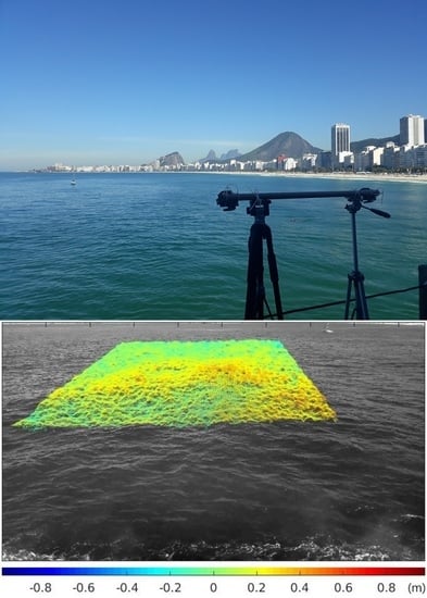
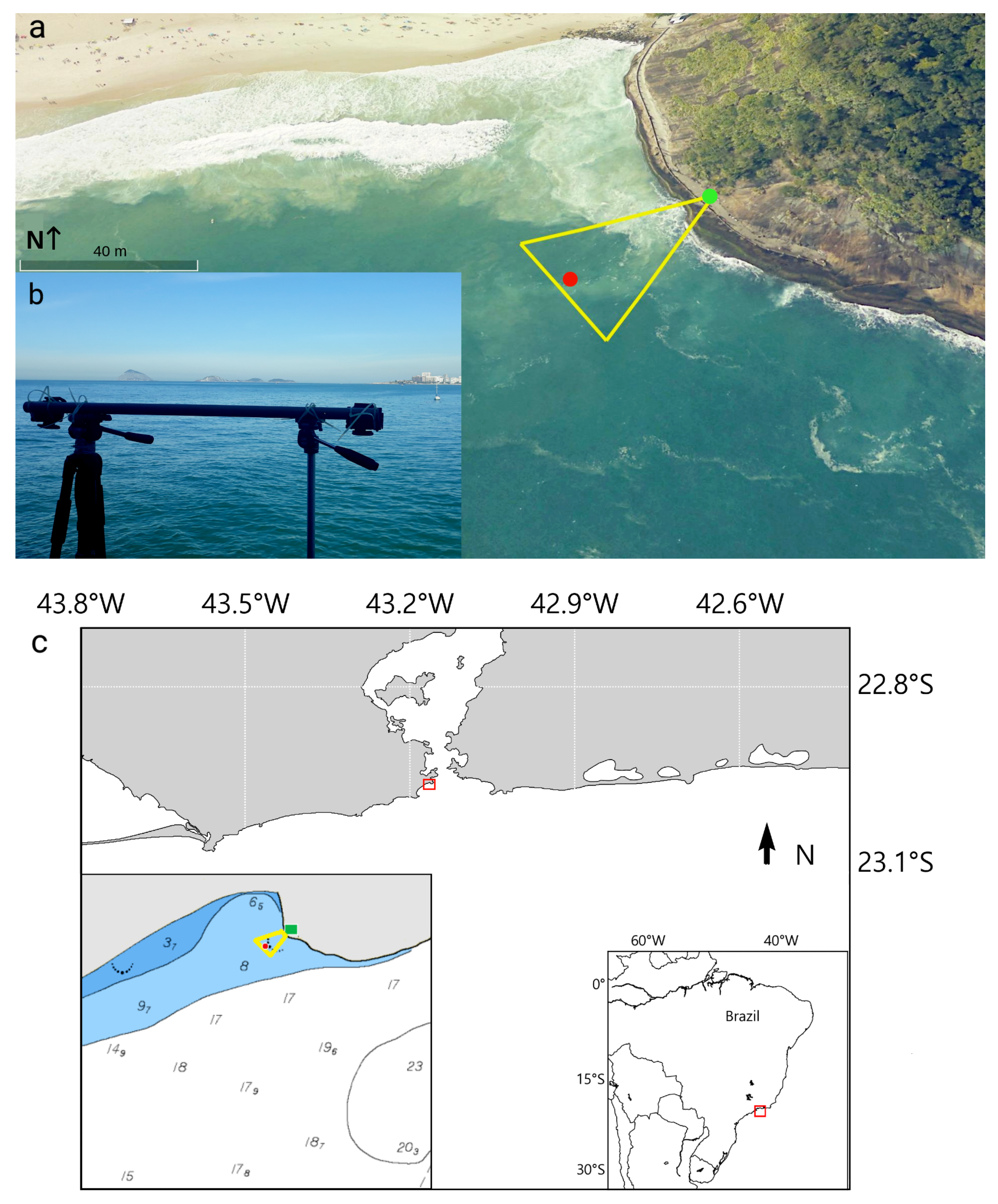
2.4. Experimental Setup and Conditions

The stereo video system using conventional smartphones was deployed in the vicinity of a sandy beach, in Rio de Janeiro, Brazil (Figure 1c). The shooting devices are two smartphones Samsung Galaxy J5 Pro, with a digital sensor type Complementary Metal Oxide Semiconductor (CMOS), acquisition rate of 30 fps, resolution of 1920 × 1080 pixels, aperture f/1.7, 13 megapixels, and focal length of 3.71 mm. This camera device was used because it has a fairly good camera on a budget phone. However, the presented methodology is not limited by any specific brand. Better performance is expected with newer and more sophisticated camera devices; the quality of the stereo video reconstruction will mostly depend on the main camera, experiment settings, and environmental conditions. The automatic focus function was disabled, and the exposure time was fixed in both cameras. Additionally, the ISO parameter was set to its lowest value and the shutter speed was set to its highest value to ensure a sharp image. This configuration is considered ideal to avoid blurred regions on the image which could hinder the pixel correlation process. Unlike conventional cameras, smartphones have compact digital sensors with poorer resolution and zooming capability, naturally limiting the accuracy of the measurements.

The smartphones were deployed 0.98 m apart on tripods in a simple and inexpensive configuration (Figure 1b). The assembly was 10 m (closest point) to 35 m (furthest point) away from the imaged area at a height of approximately 3.5 m above sea level. According to [32], ideally the ratio of the distance between cameras to the target distance should be around 0.10. For our tests, this ratio was between 0.1 in the near field, close to the stereo system, and 0.03 in the far field of view around the wave gauge position. Inside the imaged area, an RBR virtuoso pressure sensor was placed at a depth of 8.3 m, ∼34 m away from the cameras, with a sampling rate of 5 Hz. The results were derived from a one-day measurement in August 2019. Four 19-min videos with 30 Hz sample rate were recorded—resulting in 11,400 frames after subsampling to 10 Hz.

3. Results

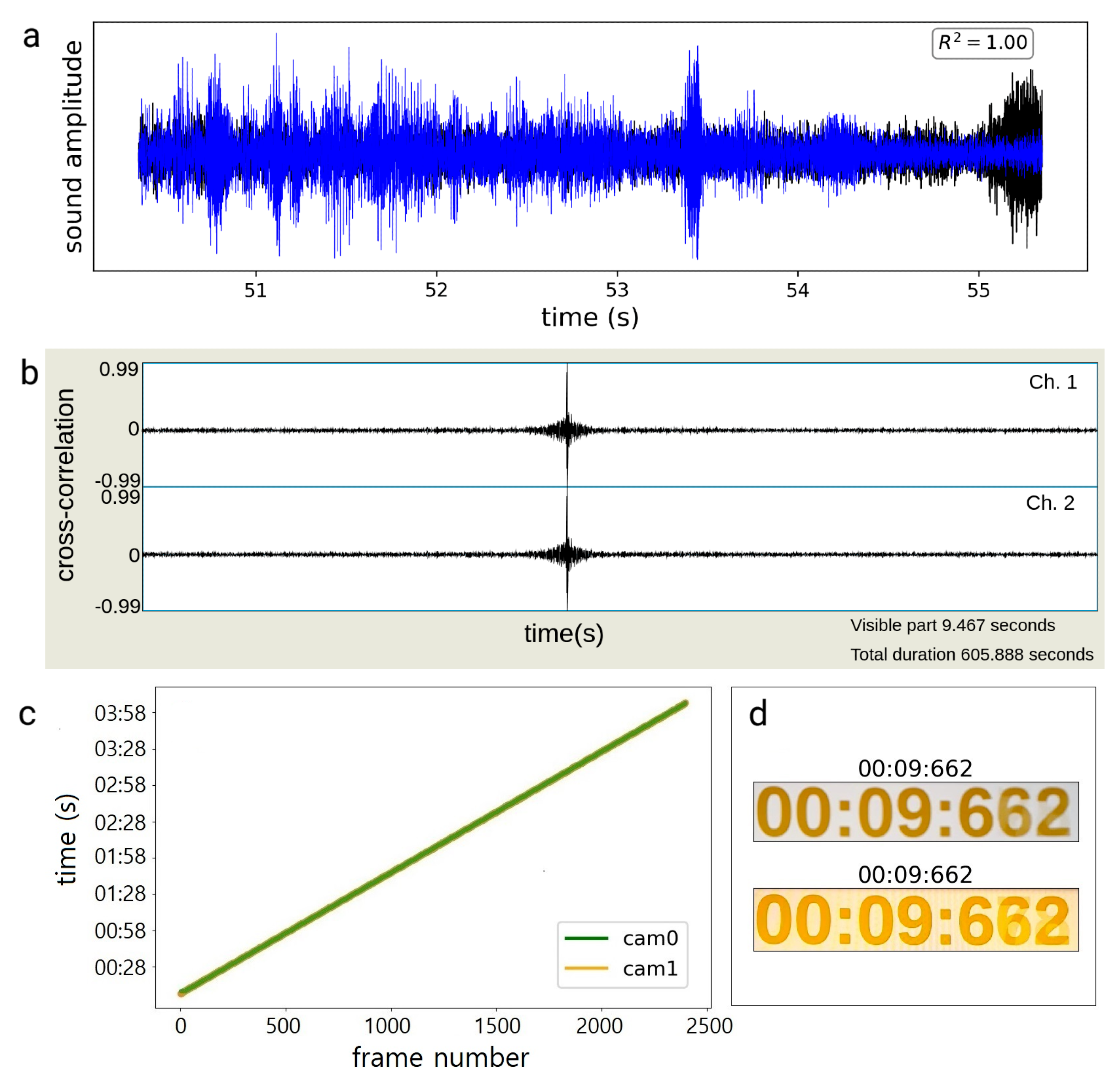
3.1. Frame Synchronization

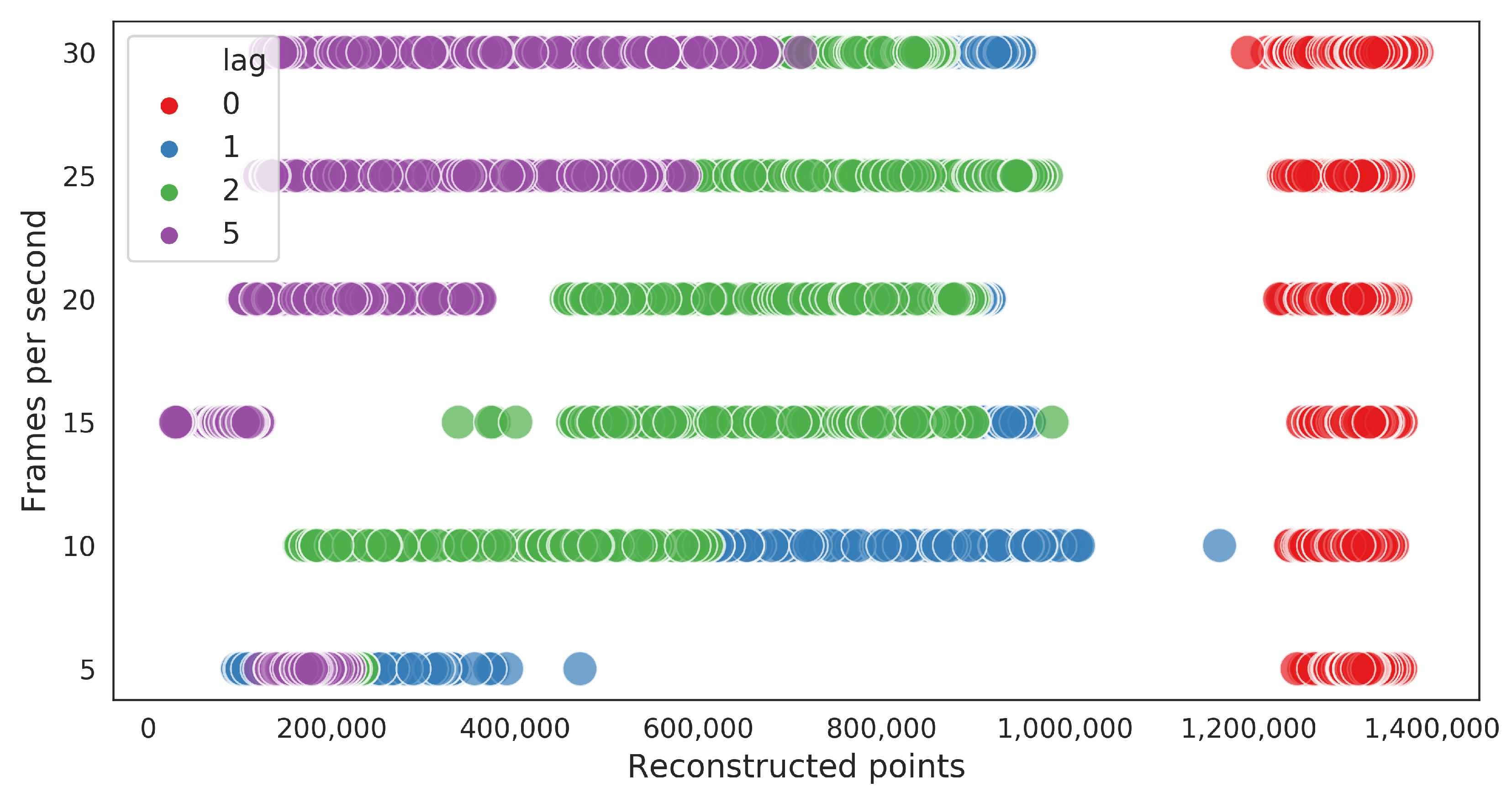
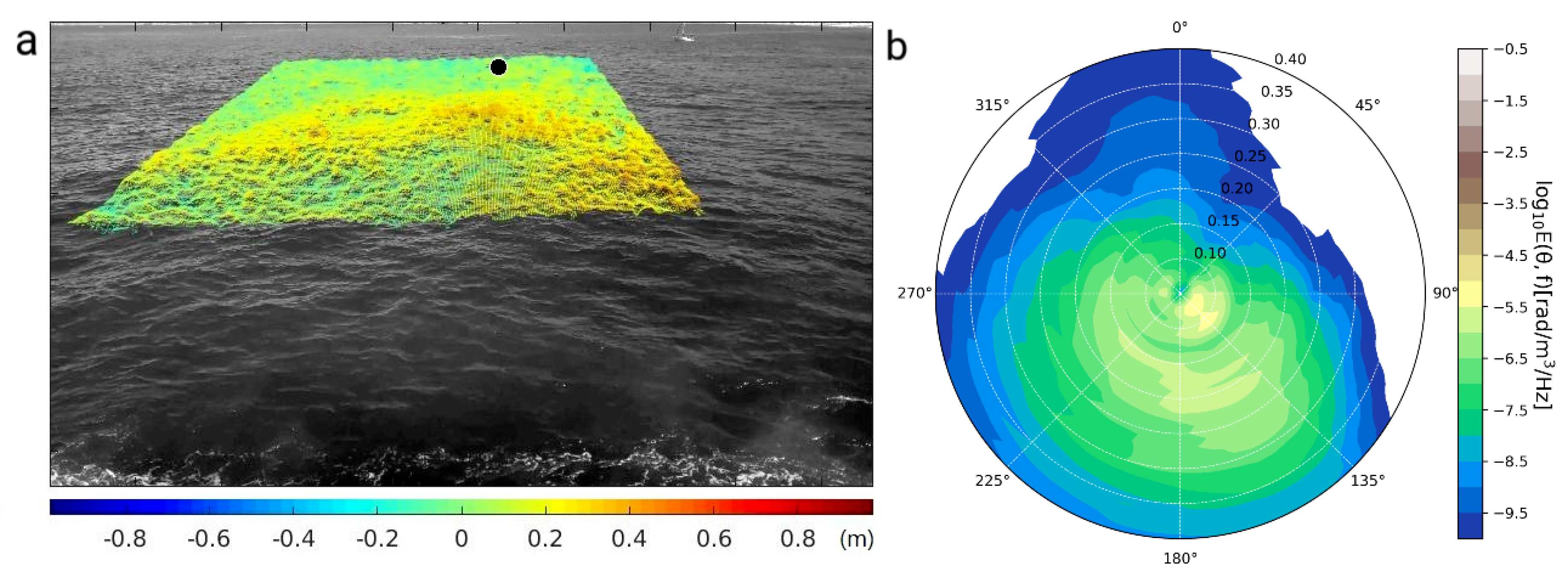
To assess the accuracy of the proposed synchronization method, a short video experiment was performed with both smartphones recording simultaneously an online atomic clock with millisecond precision. The TLCC method accurately pinpointed the time lag between records.

Figure 2a depicts an example of the time series from the two records and its corresponding cross correlation function (Figure 2b). $ar{g}_{max}$ of the cross correlation function was determined, and the two audio signals were synchronized. The correct synchronization over time is shown in Figure 2c, for which the timestamp detected by an Optical Character Recognition is the same for the two cameras in each frame. The accuracy of the method is of the order of milliseconds, as shown in Figure 2d.

We decided to exploit the epipolar constraints to evaluate the accuracy of the proposed synchronization method on real data. Indeed, if the two stereo frames are not properly synchronized, it is likely that matching features will not lie on the corresponding epipolar lines. Since WASS only searches for stereo correspondences along those lines, the amount of reconstructed points is a good proxy for the synchronization accuracy. In Figure 3, we report the test results about the total number of reconstructed points for each frame pair, performed varying the sample rate—5, 10, 15, 20, 25, and 30 fps—and an imposed frame lag—no frame lag, 1, 2, and 5; see the colors. Every video record has a length of 1 min; therefore 25,200 frames were used in all experiments. Naturally, the larger number of reconstructed points occurs with no lag—red points in Figure 3—even considering different sample rates. For lower sample rates and larger frame lags, the number of correctly reconstructed points is severely reduced. The clustering of red points on the right part of the plots, for different sample rates, is a robust indication of the quality of the synchronization method employed.

3.2. Stereo Video

Each pair of synchronized video images yielded a scatter cloud of points representing the elevation $\eta (x,y,t)$, which was gridded into a 10 × 10 m surface with 10 cm resolution (Figure 4a). The black dot represents the pressure sensor location. A stereo video system captures the space-time wave dynamics in the camera’s field of view, from which the main statistical sea state parameters can be computed—such as significant wave height (Hs), mean and peak wave period (Tm and Tp), and peak and mean wave direction (Dp and Dm).

Moreover, it is also possible to analyze the Mean Squared-Slope (MSS), the 3-D wavenumber and frequency spectrum $E(k_x,k_y,f)$, the 2-D directional spectrum $E(f,\theta )$ (as shown in Figure 4b), and the 1-D variance spectrum $E\left(f\right)$. The 3-D wavenumber and frequency spectrum is achieved by applying a 3-D Fast Fourier Transform (FFT) to convert the physical space $(x,y,t)$ into a three-dimensional spectral space. The 2-D frequency spectrum presented here is calculated from $E(k_x,k_y,f)$ by an integration along frequencies with a conversion from cartesian coordinates ($k_x,k_y$) to polar coordinates ($\theta$) [20]. The auto and cross spectra were estimated as described in [40], using Fourier transforms over time series of 5700 samples, with a 50% overlap and a Hann window. The spectra have a frequency resolution of 0.01 Hz, 44 degrees of freedom, and 22 independent windows. Significant wave height, mean, and peak wave period were computed from the 1-D frequency spectrum $E\left(f\right)$ (Figure 5b).

The 2-D directional spectrum obtained from stereo video results assumed closer characteristics with the northward swell because the location where the data was collected is more exposed to the swell components coming from south. The reconstructed zone is sheltered by the Leme Rock from waves arriving from east/northeast and limited by the beach in north/northwest portion. Therefore, the incoming wave energy can come only from west, southwest, southeast, and south (see Figure 1). In addition, it is possible to see a relative small energy coming from the north, which can be explained by a wave reflection process caused by the presence of the beach close to the reconstructed area.

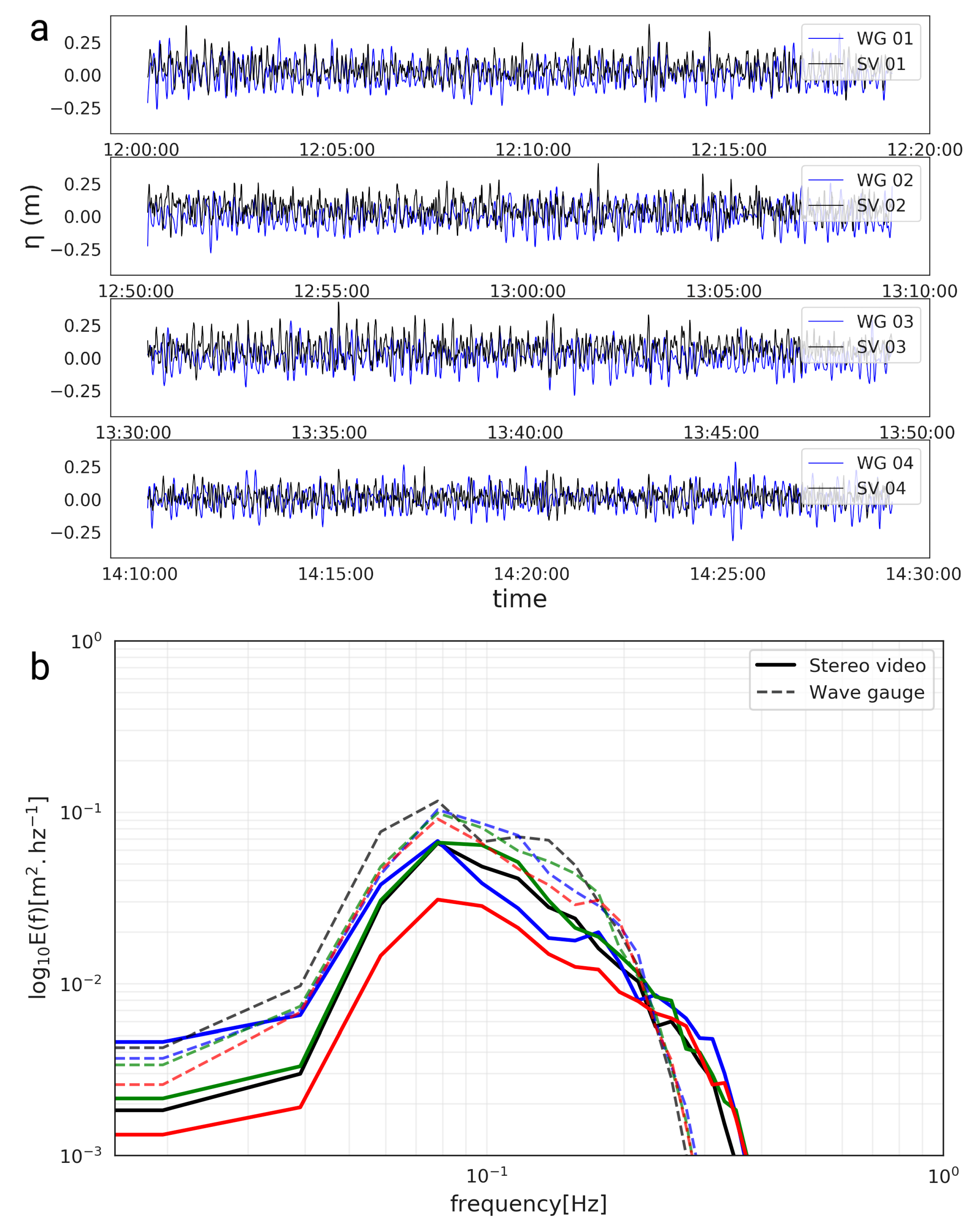
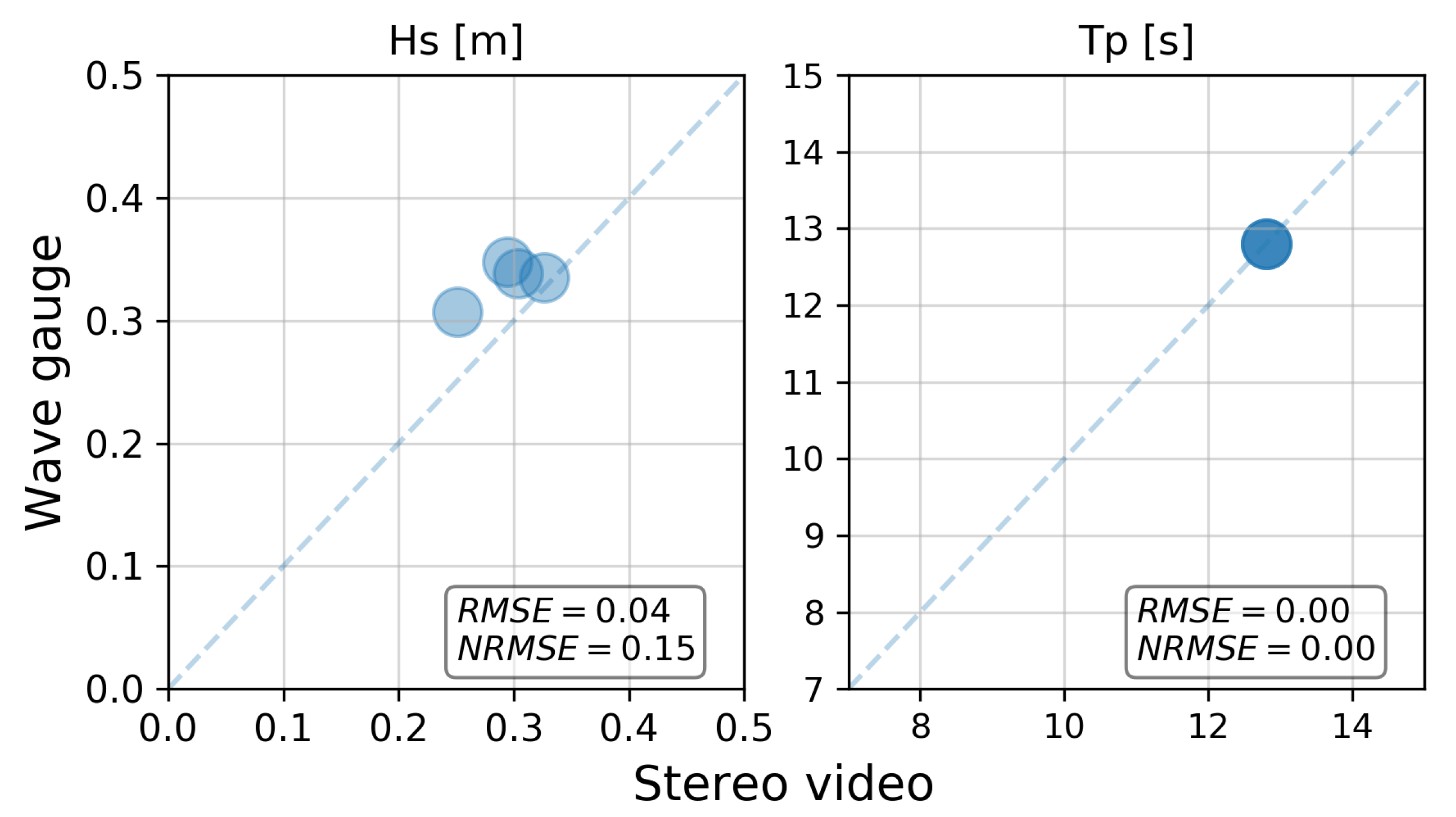
3.3. Validation against In Situ Measurements

Our main goal is to present a simple and effective way to synchronize video records from smartphones or any video device with audio built-in using a stereo system to estimate the surface elevation. The technique per se has been extensively tested under a variety of sea state conditions [14,28,29,33,34,36]. Here, to demonstrate that the proposed synchronization technique is robust, some comparisons with in situ wave measurements as ground truth are discussed.

The experimental setup can significantly influence data accuracy, particularly when simple, nonprofessional cameras are employed, as described here. Hence, to assess the proposed method, in situ measurements are essential for its validation. A comparison between the surface elevation recorded by the pressure sensor and its counterpart (approximate) position in the stereo video system is presented in Figure 5a, for 11,400 consecutive frames. The coordinates of the pressure sensor were estimated with a GPS during its mooring and identified on the stereo video image, but slight discrepancies in its position are expected.

Figure 5b shows a comparison between the 1-D frequency spectrum measured with the pressure sensor and the stereo system for a 19-min interval. Despite their overall agreement, the stereo video system underestimates the energy for frequencies lower than ∼0.15 Hz. For higher frequencies, on the other hand, the opposite pattern is observed, which might be related to the pressure sensor response. The wave-induced pressure decreases with increasing depth and more rapidly for higher frequencies. Figure 6 and

Table 1. Significant wave height ($H_s$) and peak period ($T_p$) measured with the Stereo Video System (SV) and Pressure Sensor Wave Gauge (WG) in four different moments labelled as 01, 02, 03, and 04: the Root Mean Square Error (RMSE) and bias between SV and WG are also given.

Sensor	Hs (m)	Tp (s)	RMSE${}_{\mathit{\eta }}$ (m)	Bias${}_{\mathit{\eta }}$ (m)
SV 01	0.29	12.8	0.10	−0.04
WG	0.35	12.8
SV 02	0.30	12.8	0.12	−0.05
WG	0.34	12.8
SV 03	0.33	12.8	0.12	−0.06
WG	0.33	12.8
SV 04	0.35	12.8	0.10	−0.01
WG	0.30	12.8

show the assessment of the spectral parameters $H_s$ and $T_p$, and the respective root mean square error (RMSE) between stereo video and wave gauge results. The stereo system in general underestimates $H_s$ and estimates $T_p$ very accurately.

4. Discussion

The uncertainties in the calibration processing are usually small [37]. The intrinsic calibration has been performed in controlled conditions before deployment in the field and produced a maximum error of 0.45 pixel, while the mean extrinsic calibration error was around 0.21 pixel. The identification errors of homologous points on synchronized images, however, are harder to estimate. The matching process is dependent on the image quality, the natural environmental conditions such as sun glint, water transparency, rain, and experiment setup, to name a few. In general, the matching error is small if there is enough texture on the water surfaces [9] and is minimal when the wave slope is much larger than the inclination of the stereo cameras optical axis [41]. Hence, each experiment must be carefully designed to meet the requirements of accurate 3-D estimation and accurate image matching, as reported in [29]. A good indicator of the impact of matching errors is the number of pixel matched (otherwise removed by the dense-stereo processing). Particular mismatches can occur on the edge of the matched area. To deal with those potential errors, it is recommended to consider only those points lying in the central part of the matched area [34]. For the data provided here, most of the image pixels were matched (1.4 million, as seen in Figure 3—red dots).

Furthermore, some uncertainties related to the recovery of 3-D coordinates need to be taken into account. The quantization error [15,29,42] depends on the camera cell size and pixel numbers, focal length, distance between cameras (baseline), the camera orientation, and the distance between the cameras and the target. Considering our specific configuration, the estimated root mean square quantization errors were 0.9 mm, 9.9 mm, and 1.1 mm for the x, y and z-axes, respectively—see the discussion in [42]. Figure 7b exemplifies our expected reconstruction error, as reported in [43]. For reference, [34] reported a root mean square quantization error in the z-axis of 1 cm for a high-quality stereo video system installed at 23 m above the mean sea level and 9 cm for a setup at 45 m height. However, these values are very sensitive to the cameras used, the distance from the surface, shooting angles, and sea state conditions.

An in depth discussion about the expected error and precision is described in [9,27,29,34,42,43] and references therein. In summary, assessment of stereo observations and analysis of related errors reveal that the new methodology provides meaningful data for wave measurements. We acknowledge some noise at high frequency (above about 0.5 Hz), but once it is removed, the stereo data are consistent with results provided by the nonlinear wave theory over all ranges of elevations (Figure 7a).

The error analysis presented shows a range of variables that can influence the quality of the results, which is acceptable considering that it comes from complex data, which fully describes the sea state based on 4-D sea surface information (3-D space + time). This knowledge is only accessed by specific and relatively expensive instruments, which can continuously sample an area of the ocean over time with high sample rates. Thus, given the availability of several wave measurement instruments in the market and the importance to popularize and to make feasible the wave measurements for diverse purposes, the instrument cost demand is an important parameter to consider. The price ranges for traditional stereo video acquisition systems are from 15 to 50 thousand dollars, and our system is less than 350$ if we buy two smartphones only for that. The postprocessing can be done using only open-source codes for both methods in a normal single-core computer but can be done a lot faster if parallel processing methods are adopted.

5. Conclusions

Here, we presented a simple TLCC method to synchronize stereo video acquisitions. Its performance and capability are tested by estimating the sea surface elevation and its statistical properties. The proposed methodology is considered low-cost because it does not require any dedicated equipment or software for measurements. The codes are based on open-source libraries and can be easily employed—see the video synchronization code in Appendix A. The calibration was performed using an open MATLAB toolbox, with similar tools written in Python or C++ (e.g., https:docs.opencv.org/2.4/doc/tutorials/calib3d/camera_calibration/camera_calibration.html, OpenCV camera calibration toolbox).

When compared against traditional stereo video techniques to measure surface gravity waves, it does not require a specific power supply, cables, waterproof cases, complex logistics, or dedicated batteries. Moreover, the proposed audio synchronization scheme does not require a dedicated trigger or any specific acquisition software (

Table 2. General comparative between traditional stereo video acquisition system and the proposed low-cost stereo video system.

	Traditional Stereo Video	Low-Cost Stereo Video
Video cameras	2 Wired connected dedicated cameras and 2 lens	2 Smartphones or video cameras with audio built-in
Power supply	External power supply + cables	Optional
Synchronization	Proprietary trigger box or trigger controller	Offline TLCC method
Acquisition system	Fast computer and dedicated software	Smartphones App
Cameras mounting system	Dedicated camera cases	Tripod and Smartphone support
Images quality	Higher	Lower
Storage space required	Higher	Lower (due to video compression)
Calibration procedure	Same for booth system
Fixed platform	Same for booth system
Lighting and environmental conditions	Same for both system
Postprocessing time	Near the same *

* Cross correlation and video segmentation take less than 1% of postprocessing time.

). To outline the TLCC synchronization capability, we opted for a budget smartphone; however, the main limitation of the proposed methodology remains the same as of any stereo video system, i.e., the requirement of a fixed platform or vessel near the water surface. As with similar approaches, the quality of the reconstruction is dependent on the lighting conditions, experimental setup, and camera quality. The postprocessing time is directly related to the camera’s resolution, duration of the records, and number of frames, requiring a certain amount of storage space and processing power. However, the whole procedure is easily implemented in a regular personal computer.

The stereo video reconstruction methodology proposed here was assessed against a bottom mounted pressure sensor. The root mean square error at significant wave height was $11\%$, and it was perfectly able to identify the peak period. It is worth mentioning that the wave height measured with the pressure sensor might have been attenuated because of the expected sensor response with depth. However, in ideal conditions, perfect light diffusion, and camera settings, the stereo video uncertainties could be reduced to the quantization error, of the order of millimeters. The method was deployed in a Eulerian reference system, but similar to other stereo video systems, with the correct motion correction, it could be also implemented on boats, drones, or other moving platforms.

The use of conventional, low-cost smartphones simplify the implementation of stereo video systems for multiple purposes. The results presented here are only a proof of concept that needs to be further tested in broader oceanographic conditions. Our expectation is that this nonintrusive, inexpensive, and accurate methodology will open up new and exciting possibilities in terms of wave directionality measurements, both for scientific and recreational applications.

References

1. Cox, C.; Munk, W. Measurement of the Roughness of the Sea Surface from Photographs of the Sun’s Glitter. J. Opt. Soc. Am. 1954, 44, 838–850. [Google Scholar] [CrossRef]
2. Cox, C.; Munk, W. Statistics Of The Sea Surface Derived From Sun Glitter. J. Mar. Res. 1954, 13, 198–227. [Google Scholar]
3. Monaldo, F.M.; Kasevich, R.S. Daylight Imagery of Ocean Surface Waves for Wave Spectra. J. Phys. Oceanogr. 1981, 11, 272–283. [Google Scholar] [CrossRef] [Green Version]
4. Stilwell, D., Jr. Directional energy spectra of the sea from photographs. J. Geophys. Res. (1896–1977) 1969, 74, 1974–1986. [Google Scholar] [CrossRef]
5. Stilwell, D., Jr.; Pilon, R.O. Directional spectra of surface waves from photographs. J. Geophys. Res. (1896–1977) 1974, 79, 1277–1284. [Google Scholar] [CrossRef]
6. Jähne, B.; Riemer, K.S. Two-dimensional wave number spectra of small-scale water surface waves. J. Geophys. Res. 1990, 95, 11531–11546. [Google Scholar] [CrossRef]
7. Rapizo, H.; d’Avila, V.; Violante-Carvalho, N.; Pinho, U.; Parente, C.E.; Nascimento, F. Simple Techniques for Retrieval of Wind Wave Periods and Directions from Optical Images Sequences in Wave Tanks. J. Coast. Res. 2016, 32, 1227–1234. [Google Scholar] [CrossRef]
8. Banner, M.L.; Jones, I.S.F.; Trinder, J.C. Wavenumber spectra of short gravity waves. J. Fluid Mech. 1989, 198, 321–344. [Google Scholar] [CrossRef]
9. Benetazzo, A. Measurements of short water waves using stereo matched image sequences. Coast. Eng. 2006, 53, 1013–1032. [Google Scholar] [CrossRef]
10. Mironov, A.S.; Yurovskaya, M.V.; Dulov, V.A.; Hauser, D.; Guérin, C.A. Statistical characterization of short wind waves from stereo images of the sea surface. J. Geophys. Res. Oceans 2012, 117. [Google Scholar] [CrossRef] [Green Version]
11. Shemdin, O.H.; Tran, H.M.; Wu, S.C. Directional measurement of short ocean waves with stereophotography. J. Geophys. Res. Oceans 1988, 93, 13891–13901. [Google Scholar] [CrossRef]
12. Wanek, J.; Wu, C. Automated Trinocular stereo imaging system for three-dimensional surface wave measurements. Ocean Eng. 2006, 33, 723–747. [Google Scholar] [CrossRef]
13. Banner, M.L.; Barthelemy, X.; Fedele, F.; Allis, M.; Benetazzo, A.; Dias, F.; Peirson, W.L. Linking reduced breaking crest speeds to unsteady nonlinear water wave group behavior. Phys. Rev. Lett. 2014, 112, 1–5. [Google Scholar] [CrossRef] [PubMed] [Green Version]
14. Leckler, F.; Ardhuin, F.; Peureux, C.; Benetazzo, A.; Bergamasco, F.; Dulov, V. Analysis and interpretation of frequency-wavenumber spectra of young wind waves. J. Phys. Oceanogr. 2015, 45, 2484–2496. [Google Scholar] [CrossRef]
15. Benetazzo, A.; Barbariol, F.; Bergamasco, F.; Torsello, A.; Carniel, S.; Sclavo, M. Stereo wave imaging from moving vessels: Practical use and applications. Coast. Eng. 2016, 109, 114–127. [Google Scholar] [CrossRef]
16. Alvise, B.; Francesco, B.; Filippo, B.; Sandro, C.; Mauro, S. Space-time extreme wind waves: Analysis and prediction of shape and height. Ocean Model. 2017, 113, 201–216. [Google Scholar] [CrossRef]
17. Laxague, N.; Haus, B.; Bogucki, D.; Özgökmen, T. Spectral characterization of fine-scale wind waves using shipboard optical polarimetry. J. Geophys. Res. Oceans 2015, 120, 3140–3156. [Google Scholar] [CrossRef]
18. Guimarães, P.V. Sea Surface and Energy Dissipation. Ph.D. Thesis, École centrale de Nantes, Nantes, France, 2018. [Google Scholar]
19. Schwendeman, M.S.; Thomson, J. Sharp-Crested Breaking Surface Waves Observed from a Ship-Based Stereo Video System. J. Phys. Oceanogr. 2017, 47, 775–792. [Google Scholar] [CrossRef]
20. Guimarães, P.V.; Ardhuin, F.; Sutherland, P.; Accensi, M.; Hamon, M.; Pérignon, Y.; Thomson, J.; Benetazzo, A.; Ferrant, P. A surface kinematics buoy (SKIB) for wave–current interaction studies. Ocean Sci. 2018, 14, 1449–1460. [Google Scholar] [CrossRef] [Green Version]
21. Schumacher, A. Stereophotogrammetrische Wellenaufnahmen. In Wissenschaftliche Ergebnisse Der Deutschen Atlantischen Expedition Auf Dem Forschungs- Und Vermessungss. "Meteor”. 1925–1927; Walter de Gruyter: Berlin, Germany, 1939. [Google Scholar]
22. Chase, J.L. The Directional Spectrum of a Wind Generated Sea as Determined from Data Obtained by the Stereo Wave Observation Project; New York University, College of Engineering, Research Division, Department of Meteorology and Oceanography and Engineering Statistics Group: New York, NY, USA, 1957. [Google Scholar]
23. Sugimori, Y. A study of the application of the holographic method to the determination of the directional spectrum of ocean waves. Deep Sea Res. Oceanogr. Abstr. 1975, 22, 339–350. [Google Scholar] [CrossRef]
24. Holthuijsen, L.H. Observations of the Directional Distribution of Ocean-Wave Energy in Fetch-Limited Conditions. J. Phys. Oceanogr. 1983, 13, 191–207. [Google Scholar] [CrossRef] [Green Version]
25. Gallego, G.; Benetazzo, A.; Yezzi, A.; Fedele, F. Wave Statistics and Spectra via a Variational Wave Acquisition Stereo System. In Proceedings of the International Conference on Offshore Mechanics and Arctic Engineering—OMAE, Estoril, Portugal, 15–20 June 2008. [Google Scholar]
26. Fedele, F.; Benetazzo, A.; Gallego, G.; Shih, P.C.; Yezzi, A.; Barbariol, F.; Ardhuin, F. Space-time measurements of oceanic sea states. Ocean Model. 2013, 70, 103–115. [Google Scholar] [CrossRef] [Green Version]
27. Leckler, F. Observation et Modélisation du Déferlement des Vagues. Ph.D. Thesis, Université de Bretagne Occidentale, Bretagne, France, 2013. [Google Scholar]
28. Peureux, C.; Benetazzo, A.; Ardhuin, F. Note on the directional properties of meter-scale gravity waves. Ocean Sci. 2018, 14, 41–52. [Google Scholar] [CrossRef]
29. Bergamasco, F.; Torsello, A.; Sclavo, M.; Barbariol, F.; Benetazzo, A. WASS: An open-source pipeline for 3D stereo reconstruction of ocean waves. Comput. Geosci. 2017, 107, 28–36. [Google Scholar] [CrossRef]
30. Vieira, M.; Guimarães, P.V. Measuring Sea Surface Gravity Waves Using Smartphones. In Ports 2019: Port Planning and Development; American Society of Civil Engineers: Reston, VA, USA, 2019; pp. 184–192. [Google Scholar]
31. Benetazzo, A.; Bergamasco, F.; Yoo, J.; Cavaleri, L.; Kim, S.S.; Bertotti, L.; Barbariol, F.; Shim, J.S. Characterizing the signature of a spatio-temporal wind wave field. Ocean Model. 2018, 129, 104–123. [Google Scholar] [CrossRef]
32. Benetazzo, A.; Ardhuin, F.; Bergamasco, F.; Cavaleri, L.; Guimarães, P.V.; Schwendeman, M.; Sclavo, M.; Thomson, J.; Torsello, A. On the shape and likelihood of oceanic rogue waves. Sci. Rep. 2017, 7, 8276. [Google Scholar] [CrossRef]
33. Filipot, J.F.; Guimaraes, P.; Leckler, F.; Hortsmann, J.; Carrasco, R.; Leroy, E.; Fady, N.; Accensi, M.; Prevosto, M.; Duarte, R.; et al. La Jument lighthouse: A real-scale laboratory for the study of giant waves and their loading on marine structures. Philos. Trans. R. Soc. A Math. Phys. Eng. Sci. 2019, 377, 20190008. [Google Scholar] [CrossRef] [Green Version]
34. Guimarães, P.V.; Ardhuin, F.; Bergamasco, F.; Leckler, F.; Filipot, J.F.; Shim, J.S.; Dulov, V.; Benetazzo, A. A data set of sea surface stereo images to resolve space-time wave fields. Sci. Data 2020, 7, 145. [Google Scholar] [CrossRef] [PubMed]
35. Ma, Y.; Soatto, S.; Kosecká, J.; Sastry, S. An Invitation to 3-D Vision; Springer: New York, NY, USA, 2004. [Google Scholar]
36. Benetazzo, A.; Fedele, F.; Gallego, G.; Shih, P.C.; Yezzi, A. Offshore stereo measurements of gravity waves. Coast. Eng. 2012, 64, 127–138. [Google Scholar] [CrossRef] [Green Version]
37. Bouguet, J.Y. Camera Calibration Toolbox for Matlab; Technical Report; California Institute of Technology: Pasadena, CA, USA, 2004. [Google Scholar]
38. Bracewell, R.N. The Fourier Transform and Its Applications; McGraw-Hill: New York, NY, USA, 1965. [Google Scholar]
39. Boersma, P.; Weenink, D. Praat: Doing Phonetics by Computer [Computer Program] Version 6.1.09. 2020. Available online: http://www.praat.org/ (accessed on 20 August 2018).
40. Welch, P. The use of fast Fourier transform for the estimation of power spectra: A method based on time averaging over short, modified periodograms. IEEE Trans. Audio Electroacoust. 1967, 15, 70–73. [Google Scholar] [CrossRef] [Green Version]
41. Jähne, B. Spatio-Temporal Image Processing: Theory and Scientific Applications; Springer: Berlin/Heidelberg, Germany, 1993; Volume 751. [Google Scholar]
42. Rodriguez, J.J.; Aggarwal, J.K. Stochastic analysis of stereo quantization error. IEEE Trans. Pattern Anal. Mach. Intell. 1990, 12, 467–470. [Google Scholar] [CrossRef]
43. Benetazzo, A.; Barbariol, F.; Bergamasco, F.; Torsello, A.; Carniel, S.; Sclavo, M. Observation of Extreme Sea Waves in a Space–Time Ensemble. J. Phys. Oceanogr. 2015, 45, 2261–2275. [Google Scholar] [CrossRef] [Green Version]
Figure 1. (a) The study area: yellow is the camera’s field of view, whilst the red dot depicts the position of the pressure sensor. The green dot is the stereo system located on Leme Rock. (b) Stereo-rig configuration using conventional tripods. (c) Bathymetric chart, adapted from the Brazilian Navy nautical chart 1511 and the zoom out of the study area.
Jmse 08 00831 g001
Figure 2. (a) Five-second time series from the acoustic signals (sample rate—44.1 kHz) employed to synchronize the videos: the Pearson’s coefficient R 2 calculated from approximately 5 min record is also shown. (b) Cross-correlation function with a r g m a x = 0.99 computed from two acoustic signals after synchronization. (c) Individual frame’s timestamp identified by OCR (Optical Character Recognition) from two synchronized videos. (d) Synchronized frames from both cameras identified by OCR (format minutes:seconds:milliseconds).
Jmse 08 00831 g002
Figure 3. Reconstructed points after synchronization for different sample rates—in frames per second: the color is the frame lag between records—top left corner. The red color means no lag between both cameras, whereas the purple color means a lag of five frames between cameras.
Jmse 08 00831 g003
Figure 4. (a) One snapshot of 3-D sea surface elevation map η ( x , y , t ) color coded in meters: The black dot is the location of the pressure sensor. (b) Polar plot of the 2-D directional wave spectrum E ( f , θ ) in logarithm scale estimated with the low-cost stereo video system.
Jmse 08 00831 g004
Figure 5. (a) Time series of surface elevation over a period of ∼20 min (hours:minutes:seconds). The blue line represents the pressure sensor, and the black line is the video system. (b) The E(f) 1-D frequency spectrum in log scale from a (∼20 min) interval: the colors are used to represent different records, and the line style differentiates the instruments.
Jmse 08 00831 g005
Figure 6. Spectral parameters significant wave height ( H s ) and peak period ( T p ) integrated over the frequency range of the stereo video measurements—from 0.06 Hz to 0.8 Hz: also shown are the root mean square error (RMSE) and the normalized root mean square error (NRMSE).
Jmse 08 00831 g006
Figure 7. (a) Histogram of the stereo observed (OBS) surface elevations low-pass filtered at 0.5 Hz and normalized with the standard deviation σ . Theoretical curves: Gaussian (G) probability density function (pdf) and non-Gaussian pdfs that account for skewness m 3 (GC3) and skewness m 3 and kurtosis m 4 (CG4). (b) Quantization error map for the sea surface elevations (z-axis).
Jmse 08 00831 g007