
Multiple Evidence for Climate Patterns Influencing Ecosystem Productivity across Spatial Gradients in the Venice Lagoon


Abstract
:1. Introduction
2. Methods
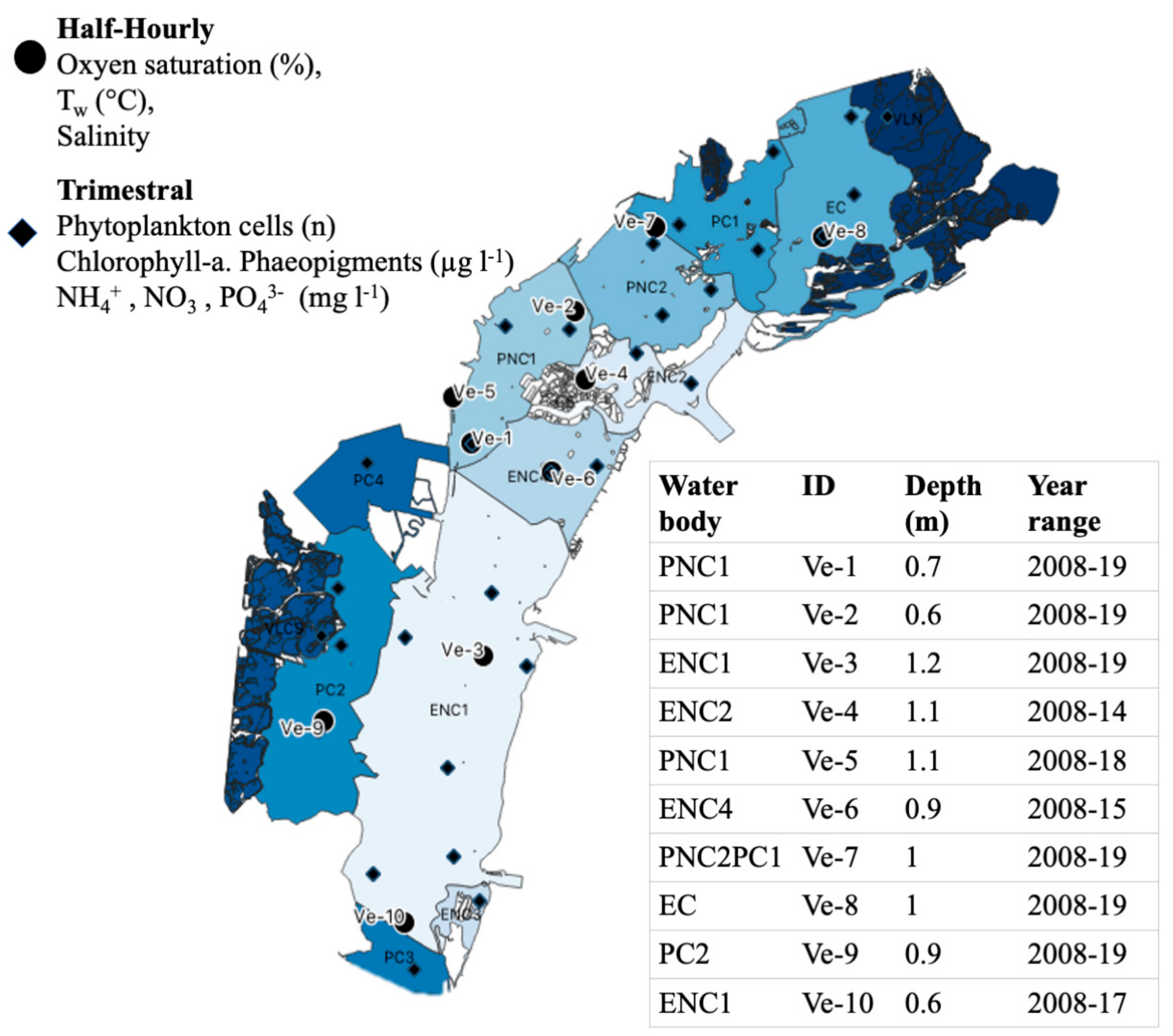
2.1. Study Site
2.2. Environmental Data
2.3. Climate Effects
2.4. Ecological Responses
Production and Respiration in the System
3. Results
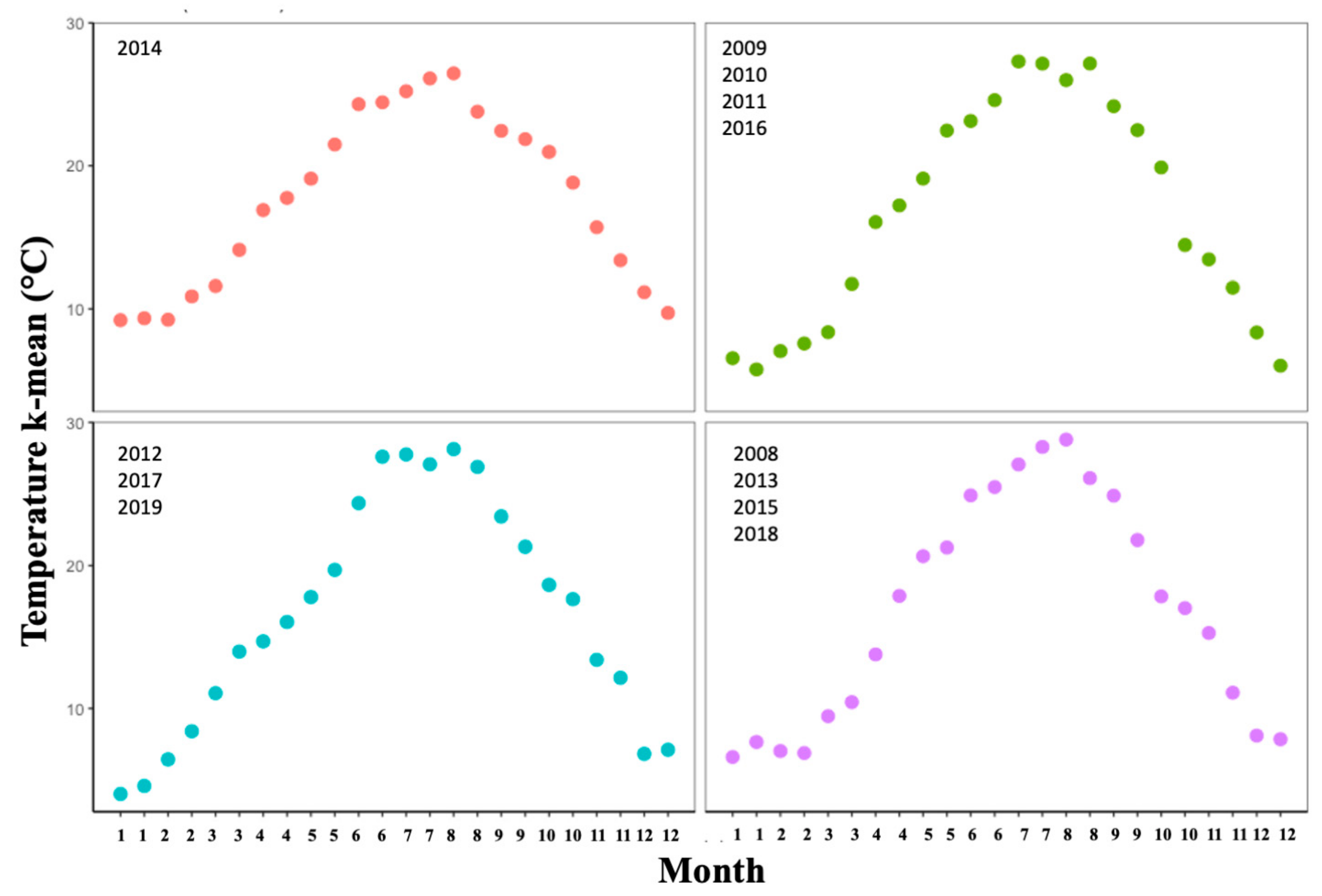
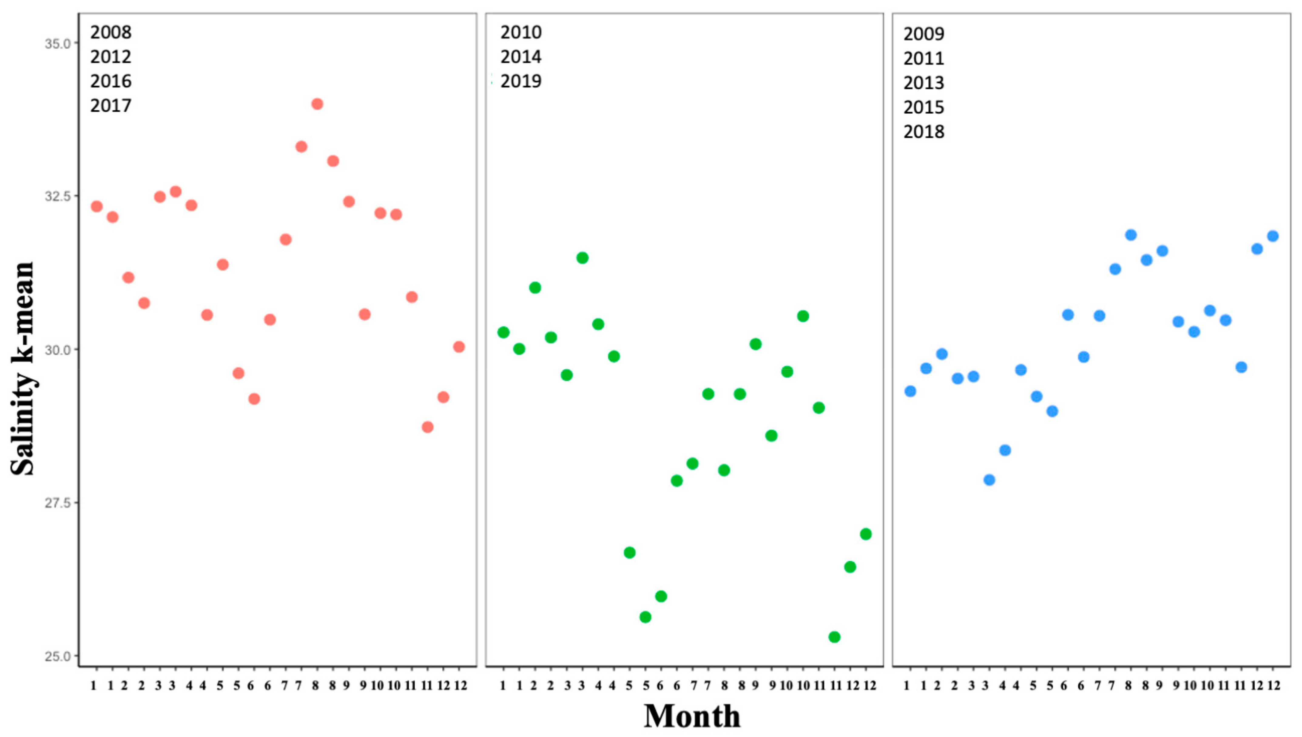
3.1. Climate: Temporal Effects
3.2. Climate: Spatial Effects
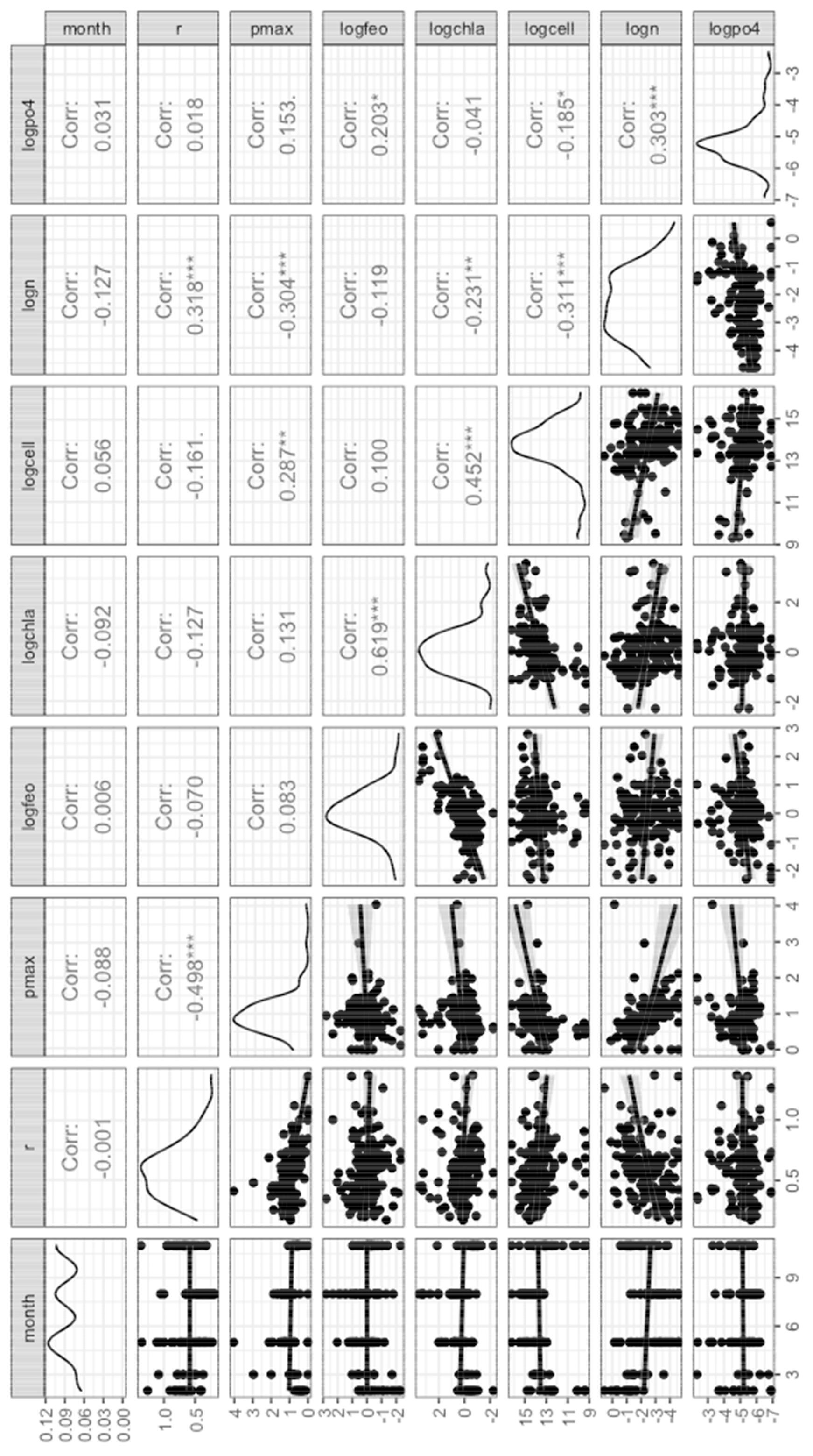
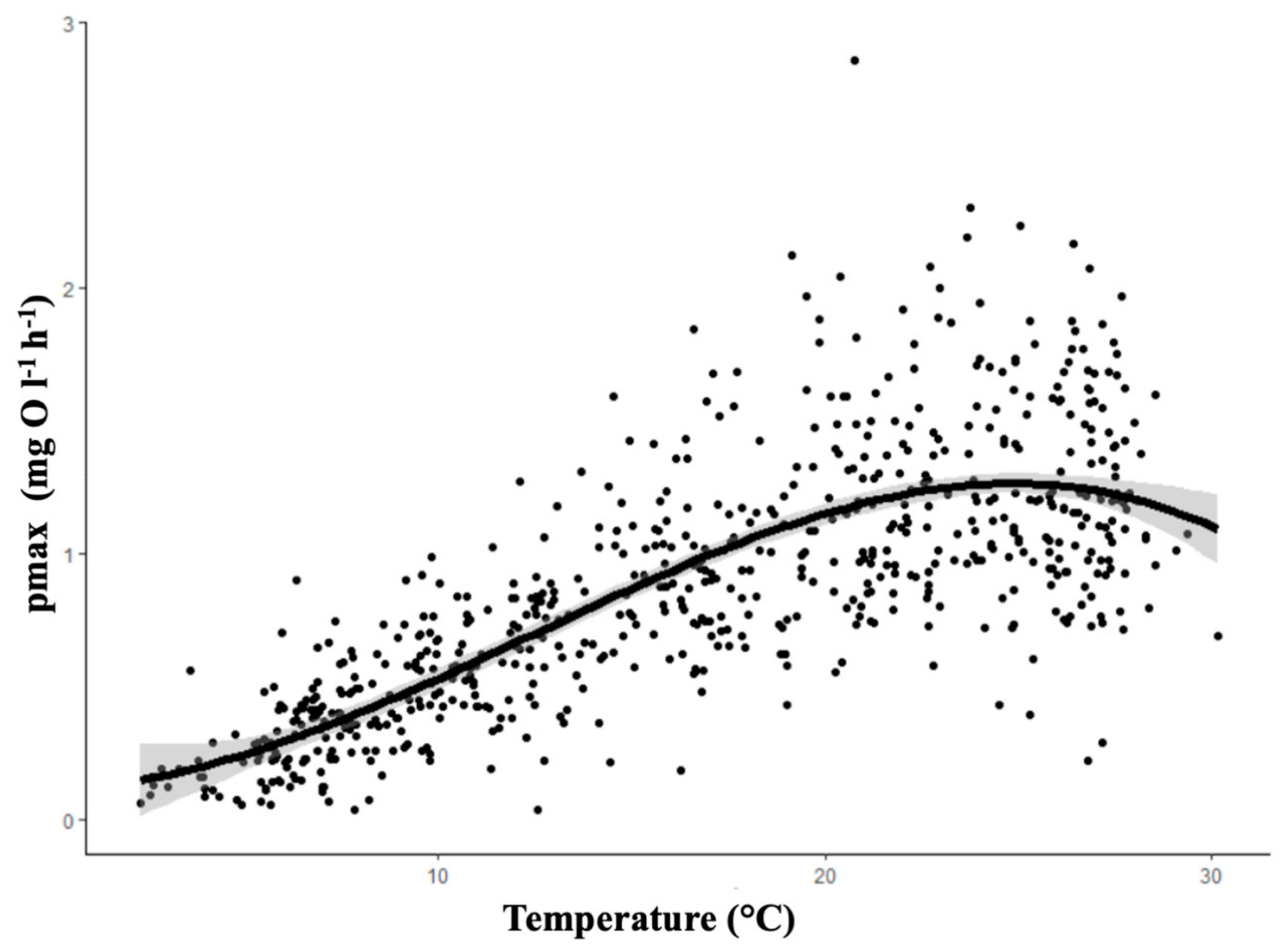
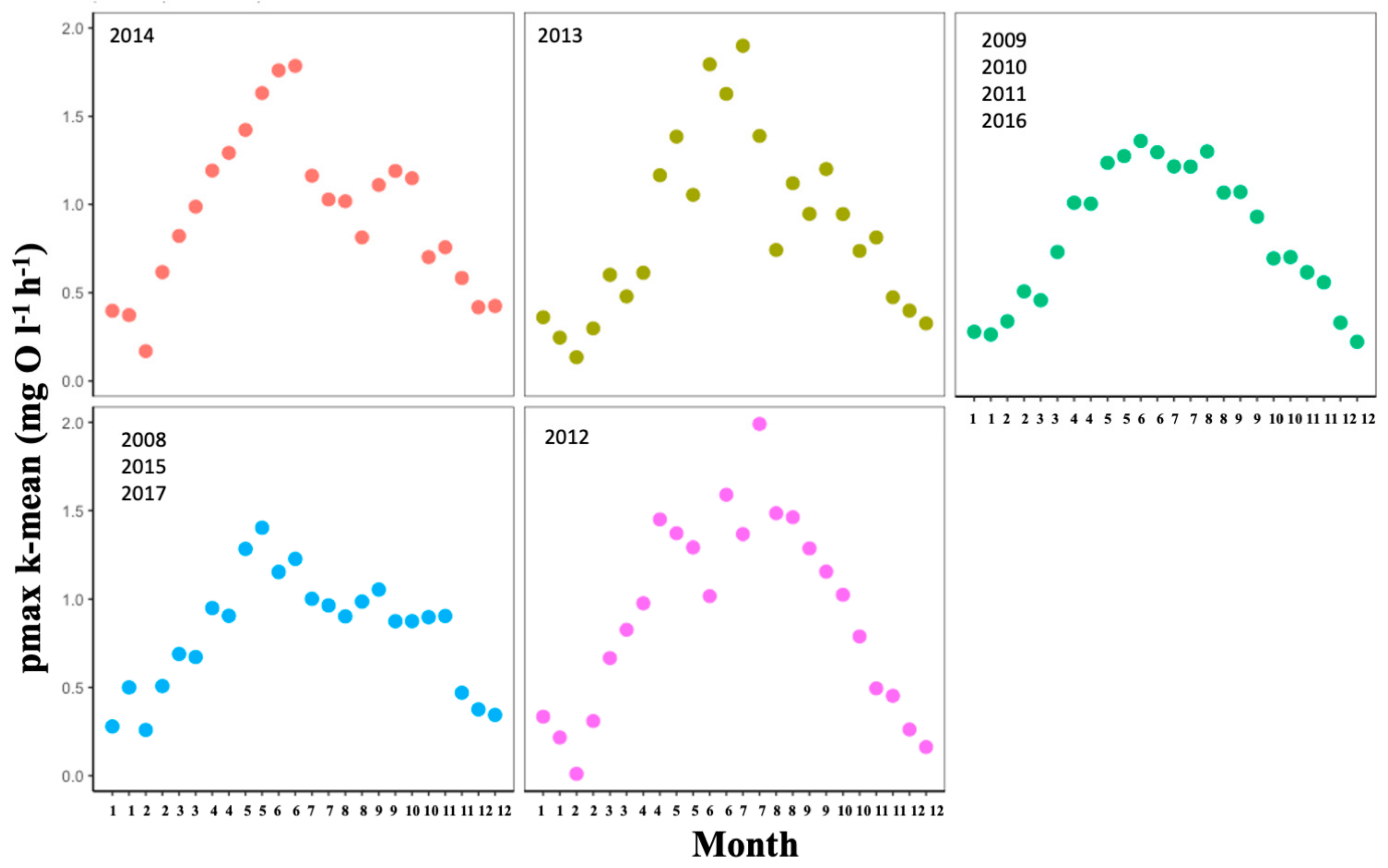
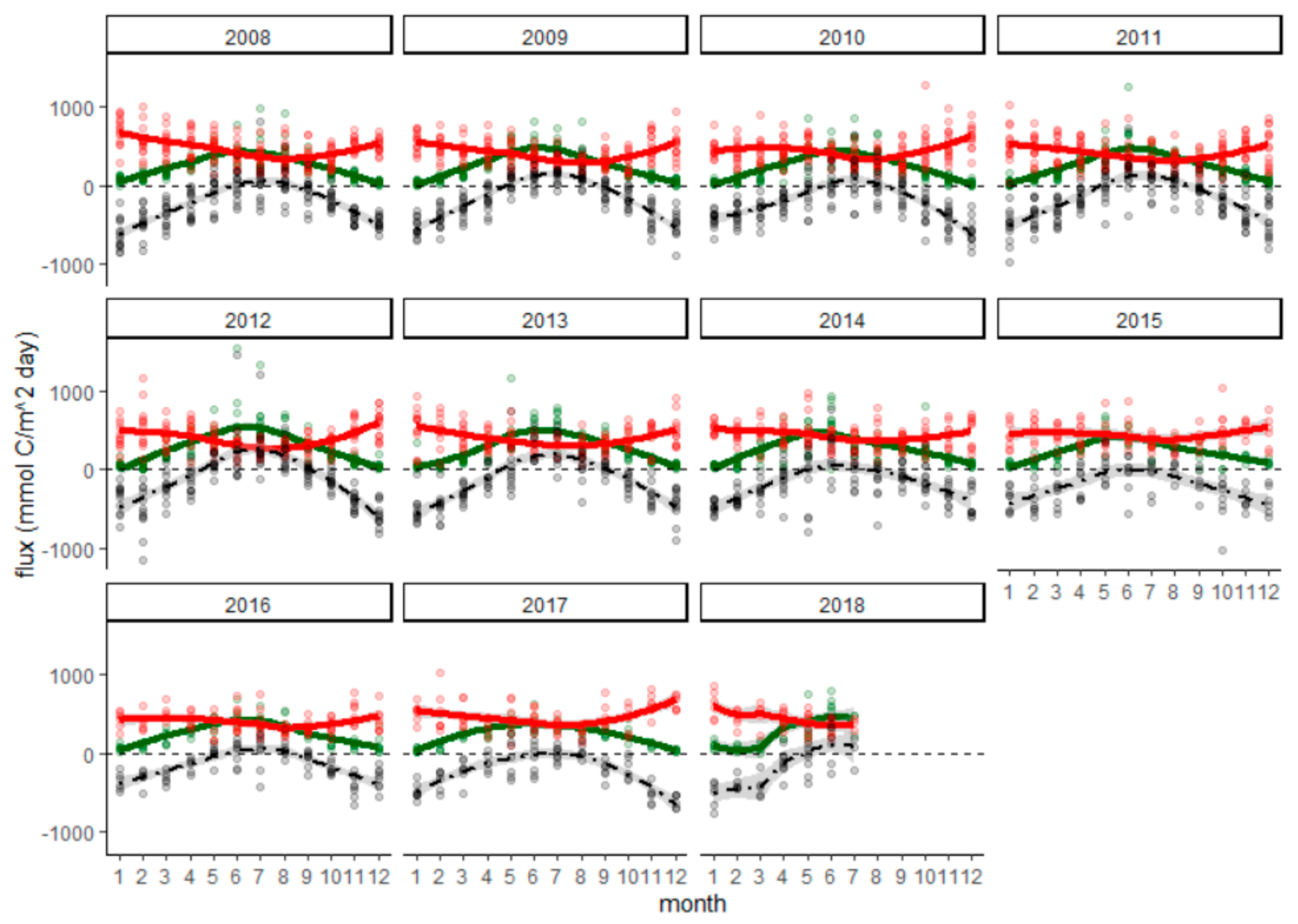
3.3. Production & Respiration
4. Discussion
Climate
5. Conclusions
Supplementary Materials
Author Contributions
Funding
Institutional Review Board Statement
Informed Consent Statement
Data Availability Statement
Acknowledgments
Conflicts of Interest
References
- Rogelj, J.; Luderer, G.; Pietzcker, R.C.; Kriegler, E.; Schaeffer, M.; Krey, V.; Riahi, K. Energy system transformations for limiting end-of-century warming to below 1.5 °C. Nat. Clim. Chang. 2015, 5, 519–527. [Google Scholar] [CrossRef]
- IPCC. IPCC Special Report on the Ocean and Cryosphere in a Changing Climate; United Nations Intergovernmental Panel on Climate Change: Geneva, Switzerland, 2019; Available online: https://www.ipcc.ch/srocc/ (accessed on 1 February 2021).
- Brierley, C.; Koch, A.; Ilyas, M.; Wennyk, N.; Kikstra, J. Half the world’s population already experiences years 1.5 °C warmer than preindustrial. EarthArXiv 2019. [Google Scholar] [CrossRef] [Green Version]
- Liu, W.; Huang, B.; Thorne, P.; Banzon, V.F.; Zhang, H.-M.; Freeman, E.; Lawrimore, J.; Peterson, T.C.; Smith, T.; Woodruff, S. Extended reconstructed sea surface temperature version 4 (ERSST.v4): Part II. Parametric and structural uncertainty estimations. J. Clim. 2015, 28, 931–951. [Google Scholar] [CrossRef]
- Huang, B.; Banzon, V.F.; Freeman, E.; Lawrimore, J.; Liu, W.; Peterson, T.C.; Smith, T.M.; Thorne, P.W.; Woodruff, S.D.; Zhang, H.M. Extended reconstructed sea surface temperature version 4 (ERSST.v4). Part I: Upgrades and intercomparisons. J. Clim. 2015, 28, 911–930. [Google Scholar] [CrossRef] [Green Version]
- Huang, B.; Thorne, P.; Smith, T.M.; Liu, W.; Lwrimore, J.; Banzon, V.F.; Zhang, H.-M.; Peterson, T.C.; Menne, M. Further exploring and quantifying uncertainties for extended reconstructed sea surface temperature (ERSST) Version 4 (v4). J. Clim. 2016, 4, 3119–3142. [Google Scholar] [CrossRef]
- Nykjaer, L. Mediterranean Sea surface warming 1985–2006. Clim. Res. 2009, 39, 11–17. [Google Scholar] [CrossRef]
- Elliott, M.; Quintino, V. The estuarine quality paradox, environmental homeostasis and the difficulty of detecting anthropogenic stress in naturally stressed areas. Mar. Pollut. Bull. 2007, 54, 640–645. [Google Scholar] [CrossRef] [PubMed]
- Scanes, E.; Scanes, P.R.; Ross, P.M. Climate change rapidly warms and acidifies Australian estuaries. Nat. Commun. 2020, 11, 1–11. [Google Scholar] [CrossRef] [Green Version]
- Pesce, M.; Critto, A.; Torresan, S.; Giubilato, E.; Santini, M.; Zirino, A.; Ouyang, W.; Marcomini, A. Modelling climate change impacts on nutrients and primary production in coastal waters. Sci. Total Environ. 2018, 628–629, 919–937. [Google Scholar] [CrossRef] [PubMed]
- Mahaffey, C.; Palmer, M.; Greenwood, N.; Sharples, J. Impacts of climate change on dissolved oxygen concentration relevant to the coastal and marine environment around the UK. MCCIP Sci. Rev. 2020, 2020, 31–53. [Google Scholar] [CrossRef]
- Lloret, J.; Marín, A.; Marín-Guirao, L. Is coastal lagoon eutrophication likely to be aggravated by global climate change? Estuar. Coast. Shelf Sci. 2008, 78, 403–412. [Google Scholar] [CrossRef]
- Trombetta, T.; Vidussi, F.; Mas, S.; Parin, D.; Simier, M.; Mostajir, B. Water temperature drives phytoplankton blooms in coastal waters. PLoS ONE 2019, 14, 1–28. [Google Scholar] [CrossRef] [PubMed] [Green Version]
- Chapin, F.S.; Woodwell, G.M.; Randerson, J.T.; Rastetter, E.B.; Lovett, G.M.; Baldocchi, D.D.; Clark, D.A.; Harmon, M.E.; Schimel, D.S.; Valentini, R.; et al. Reconciling carbon-cycle concepts, terminology, and methods. Ecosystems 2006, 9, 1041–1050. [Google Scholar] [CrossRef] [Green Version]
- Umgiesser, G.; Ferrarin, C.; Cucco, A.; De Pascalis, F.; Bellafiore, D.; Ghezzo, M.; Bajo, M. Comparative hydrodynamics of 10 Mediterranean lagoons by means of numerical modeling. J. Geophys. Res. Ocean. 2014, 119, 2212–2226. [Google Scholar] [CrossRef]
- Ghezzo, M.; Sarretta, A.; Sigovini, M.; Guerzoni, S.; Tagliapietra, D.; Umgiesser, G. Modeling the inter-annual variability of salinity in the lagoon of Venice in relation to the water framework directive typologies. Ocean Coast. Manag. 2011, 54, 706–719. [Google Scholar] [CrossRef] [Green Version]
- Pérez-Ruzafa, A.; Marcos, C.; Pérez-Ruzafa, I.M.; Pérez-Marcos, M. Coastal lagoons: “transitional ecosystems” between transitional and coastal waters. J. Coast. Conserv. 2011, 15, 369–392. [Google Scholar] [CrossRef]
- Solidoro, C.; Bandelj, V.; Bernardi, F.A.; Camatti, E.; Ciavatta, S.; Cossarini, G.; Facca, C.; Franzoi, P.; Libralato, S.; Canu, D.M.; et al. Response of the Venice Lagoon ecosystem to natural and anthropogenic pressures over the last 50 years. Coast. Lagoons Crit. Habitats Environ. Chang. 2010, 8, 483–511. [Google Scholar] [CrossRef]
- Ferrarin, C.; Bajo, M.; Bellafiore, D.; Cucco, A.; De Pascalis, F.; Ghezzo, M.; Umgiesser, G. Toward homogenization of Mediterranean lagoons and their loss of hydrodiversity. Geophys. Res. Lett. 2014, 41, 5935–5941. [Google Scholar] [CrossRef]
- Critto, A.; Rizzi, J.; Gottardo, S.; Marcomini, A. Assessing the environmental quality of the venice lagoon waters using the E-QUALITY software tool. Environ. Eng. Manag. J. 2013, 12, 211–218. [Google Scholar] [CrossRef]
- Ghezzo, M.; Pellizzato, M.; De Pascalis, F.; Silvestri, S.; Umgiesser, G. Natural resources and climate change: A study of the potential impact on Manila clam in the Venice lagoon. Sci. Total Environ. 2018, 645, 419–430. [Google Scholar] [CrossRef]
- Ferrari, G.; Petrizzo, A.; Badetti, C.; Pisarroni, E.; Berton, A. La Rete di Monitoraggio SAMANET della Qualita’delle Acque della Laguna di Venezia; Magistrale alle Acque di Venezia: Venice, Italy, 2008. [Google Scholar]
- Hartigan, J.A.; Wong, M.A. Algorithm AS 136: A K-means clustering algorithm. J. R. Stat. Soc. Ser. C Appl. Stat. 1979, 28, 100–108. [Google Scholar] [CrossRef]
- Thorndike, R.L. Who belongs in the family? Psychometrika 1953. [Google Scholar] [CrossRef]
- Ciavatta, S.; Pastres, R.; Badetti, C.; Ferrari, G.; Beck, M.B. Estimation of phytoplanktonic production and system respiration from data collected by a real-time monitoring network in the Lagoon of Venice. Ecol. Modell. 2008, 212, 28–36. [Google Scholar] [CrossRef]
- Odum, E.P.; Barrett, G.W. Fundamentals of Ecology, 3rd ed.; W. B. Saunders Company: Philadelphia, PA, USA, 1971. [Google Scholar]
- Amos, C.L.; Umgiesser, G.; Ghezzo, M.; Kassem, H.; Ferrarin, C. Sea surface temperature trends in venice lagoon and the adjacent waters. J. Coast. Res. 2017, 33, 385–395. [Google Scholar] [CrossRef]
- Umgiesser, G.; Canu, D.M.; Cucco, A.; Solidoro, C. A finite element model for the Venice Lagoon. Development, set up, calibration and validation. J. Mar. Syst. 2004, 51, 123–145. [Google Scholar] [CrossRef]
- Pivato, M.; Carniello, L.; Viero, D.P.; Soranzo, C.; Defina, A.; Silvestri, S. Remote sensing for optimal estimation of water temperature dynamics in shallow tidal environments. Remote Sens. 2020, 12, 51. [Google Scholar] [CrossRef] [Green Version]
- Boyd, P.W.; Rynearson, T.A.; Armstrong, E.A.; Fu, F.; Hayashi, K.; Hu, Z.; Hutchins, D.A.; Kudela, R.M.; Litchman, E.; Mulholland, M.R.; et al. Marine phytoplankton temperature versus growth responses from polar to tropical waters—Outcome of a scientific community-wide study. PLoS ONE 2013, 8, e0063091. [Google Scholar] [CrossRef] [Green Version]
- Baker, K.G.; Robinson, C.M.; Radford, D.T.; McInnes, A.S.; Evenhuis, C.; Doblin, M.A. Thermal performance curves of functional traits aid understanding of thermally induced changes in diatom-mediated biogeochemical fluxes. Front. Mar. Sci. 2016, 3, 1–14. [Google Scholar] [CrossRef] [Green Version]
- Anthony, A.; Atwood, J.; August, P.; Byron, C.; Cobb, S.; Foster, C.; Fry, C.; Gold, A.; Hagos, K.; Heffner, L.; et al. Coastal lagoons and climate change: Ecological and social ramifications in U.S. Atlantic and Gulf coast ecosystems. Ecol. Soc. 2009, 14, 108. [Google Scholar] [CrossRef]
- Solidoro, C.; Pastres, R.; Cossarini, G. Nitrogen and plankton dynamics in the lagoon of Venice. Ecol. Modell. 2005, 184, 103–123. [Google Scholar] [CrossRef]
- Duarte, C.M.; Regaudie-De-Gioux, A.; Arrieta, J.M.; Delgado-Huertas, A.; Agustí, S. The oligotrophic ocean is heterotrophic. Ann. Rev. Mar. Sci. 2013, 5, 551–569. [Google Scholar] [CrossRef]
- Wiegner, T.N.; Seitzinger, S.P.; Breitburg, D.L.; Sanders, J.G. The effects of multiple stressors on the balance between autotrophic and heterotrophic processes in an estuarine system. Estuaries 2003, 26, 352–364. [Google Scholar] [CrossRef]
- Lovato, T.; Ciavatta, S.; Brigolin, D.; Rubino, A.; Pastres, R. Modelling dissolved oxygen and benthic algae dynamics in a coastal ecosystem by exploiting real-time monitoring data. Estuar. Coast. Shelf Sci. 2013, 119, 17–30. [Google Scholar] [CrossRef]
- Bandelj, V.; Socal, G.; Park, Y.S.; Lek, S.; Coppola, J.; Camatti, E.; Capuzzo, E.; Milani, L.; Solidoro, C. Analysis of multitrophic plankton assemblages in the Lagoon of Venice. Mar. Ecol. Prog. Ser. 2008, 368, 23–40. [Google Scholar] [CrossRef]
- Moore, C.M.; Mills, M.M.; Langlois, R.; Milne, A.; Achterberg, E.P.; La Roche, J.; Geider, R.J. Relative influence of nitrogen and phosphorus availability on phytoplankton physiology and productivity in the oligotrophic sub-tropical North Atlantic Ocean. Limnol. Oceanogr. 2008, 53, 291–305. [Google Scholar] [CrossRef]
- Libralato, S.; Pastres, R.; Pranovi, F.; Raicevich, S.; Granzotto, A.; Giovanardi, O.; Torricelli, P. Comparison between the energy flow networks of two habitats in the Venice Lagoon. Mar. Ecol. 2002, 23, 228–236. [Google Scholar] [CrossRef]
- Sfriso, A.; Curiel, D.; Rismondo, A. The lagoon of Venice. Flora Veg. Ital. Transit. Water Syst. 2009, 17–80. [Google Scholar]
- Silva, J.; Barrote, I.; Costa, M.M.; Albano, S.; Santos, R. Physiological responses of Zostera marina and Cymodocea nodosa to light-limitation stress. PLoS ONE 2013, 8, e0081058. [Google Scholar] [CrossRef] [PubMed]
- Brigolin, D.; Facca, C.; Franco, A.; Franzoi, P.; Pastres, R.; Sfriso, A.; Sigovini, M.; Soldatini, C.; Tagliapietra, D.; Torricelli, P.; et al. Linking food web functioning and habitat diversity for an ecosystem based management: A Mediterranean lagoon case-study. Mar. Environ. Res. 2014, 97, 58–66. [Google Scholar] [CrossRef]
- Sfriso, A.; Facca, C.; Bonometto, A.; Boscolo, R. Compliance of the macrophyte quality index (MaQI) with the WFD (2000/60/EC) and ecological status assessment in transitional areas: The Venice lagoon as study case. Ecol. Indic. 2014, 46, 536–547. [Google Scholar] [CrossRef]
- Bernardi-Aubry, F.; Acri, F.; Scarpa, G.M.; Braga, F. Phytoplankton—Macrophyte interaction in the lagoon. Water 2020, 12, 2810. [Google Scholar] [CrossRef]
- McGlathery, K.J.; Anderson, I.C.; Tyler, A.C. Magnitude and variability of benthic and pelagic metabolism in a temperate coastal lagoon. Mar. Ecol. Prog. Ser. 2001, 216, 1–15. [Google Scholar] [CrossRef]
- Umgiesser, G. The impact of operating the mobile barriers in Venice (MOSE) under climate change. J. Nat. Conserv. 2020, 54, 125783. [Google Scholar] [CrossRef]


| Type | Code | Name | Surface (km2) |
|---|---|---|---|
| Polyhaline confined | PC1 | Dese | 18 |
| Polyhaline confined | PC2 | Millecampi Teneri | 37 |
| Polyhaline confined | PC3 | Val di Brenta | 7 |
| Polyhaline confined | PC4 | Teneri | 10 |
| Euhaline confined | EC | Palude Maggiore | 40 |
| Euhaline not confined | ENC1 | Centro Sud | 106 |
| Euhaline not confined | ENC2 | Lido | 10 |
| Euhaline not confined | ENC3 | Chioggia | 3 |
| Euhaline not confined | ENC4 | Sacca Sessola | 24 |
| Polyhaline not confined | PNC1 | Marghera | 28 |
| Polyhaline not confined | PNC2 | Tessera | 25 |
| Month | January | February | March | April | May | June | July | August | September | October | November | December |
|---|---|---|---|---|---|---|---|---|---|---|---|---|
| Estimate (r) (mean ± SD) | 0.729 ± 0.527 | 0.703 ± 0.505 | 0.663 ± 0.492 | 0.643 ± 0.440 | 0.588 ± 0.389 | 0.508 ± 0.355 | 0.437 ± 0.311 | 0.421 ± 0.323 | 0.483 ± 0.349 | 0.555 ± 0.408 | 0.707 ± 0.491 | 0.733 ± 0.502 |
| RSE (r) (mean ± SD) | 0.225 ± 0.194 | 0.297 ± 0.221 | 0.389 ± 0.315 | 0.594 ± 0.6 | 0.726 ± 0.520 | 0.950 ± 0.651 | 1.02 ± 0.609 | 0.977 ± 0.540 | 0.7 ± 0.502 | 0.503 ± 0.483 | 0.275 ± 0.212 | 0.219 ± 0.145 |
| Estimate (pmax) (mean ± SD) | 0.323 ± 0.199 | 0.381 ± 0.223 | 0.674 ± 0.292 | 1.041 ± 0.363 | 1.292 ± 0.435 | 1.380 ± 0.465 | 1.291 ± 0.451 | 1.170 ± 0.384 | 1.071 ± 0.334 | 0.831 ± 0.353 | 0.619 ± 0.258 | 0.336 ± 0.197 |
| Year | EC (t CO2eq ha−1 Year−1) | ENC1 (t CO2eq ha−1 Year−1) | ENC2 (t CO2eq ha−1 Year−1) | ENC4 (t CO2eq ha−1 Year−1) | PC2 (t CO2eq ha−1 Year−1) | PNC1 (t CO2eq ha−1 Year−1) | PNC2PC1 (t CO2eq ha−1 Year−1) | Median Whole Lagoon Area (t CO2eq) |
|---|---|---|---|---|---|---|---|---|
| 2008 | −40.8 | −19.9 | −47.6 | −15.5 | −43.7 | −26.5 | −61 | −152,296 |
| 2009 | −22.2 | −15.9 | −37.5 | −8.4 | −32.5 | −31.2 | −32.3 | −116,376 |
| 2010 | −16.9 | −21.4 | −50.4 | −0.8 | −38.3 | −27.3 | −63.2 | −101,833 |
| 2011 | −42.2 | −11.9 | −30.9 | 0.6 | −33.4 | −24.1 | −43.3 | −115,482 |
| 2012 | −10.4 | −7.9 | −29.4 | −2.7 | −39.3 | −11.9 | −26.2 | −44,667 |
| 2013 | −31.5 | −12.3 | −30.5 | −5.5 | NA | −25.8 | −28.9 | −102,033 |
| 2014 | −38.2 | −12.3 | −20.2 | −1.5 | NA | −30.5 | −58.5 | −94,704 |
| 2015 | −35.5 | −14.4 | NA | NA | NA | −30.6 | −46.2 | −122,725 |
| 2016 | −23.6 | −19 | NA | NA | NA | −38.9 | −18.9 | −79,661 |
| 2017 | −25.2 | −28.9 | NA | NA | NA | −30.9 | −33.7 | −111,570 |
| Median whole water body (t CO2eq) | −9053 | −20,426 | −5557 | −1472 | −19,335 | −9261 | −22,784 | −107,850 |
Publisher’s Note: MDPI stays neutral with regard to jurisdictional claims in published maps and institutional affiliations. |
© 2021 by the authors. Licensee MDPI, Basel, Switzerland. This article is an open access article distributed under the terms and conditions of the Creative Commons Attribution (CC BY) license (http://creativecommons.org/licenses/by/4.0/).
Share and Cite
Bertolini, C.; Royer, E.; Pastres, R. Multiple Evidence for Climate Patterns Influencing Ecosystem Productivity across Spatial Gradients in the Venice Lagoon. J. Mar. Sci. Eng. 2021, 9, 363. https://doi.org/10.3390/jmse9040363
Bertolini C, Royer E, Pastres R. Multiple Evidence for Climate Patterns Influencing Ecosystem Productivity across Spatial Gradients in the Venice Lagoon. Journal of Marine Science and Engineering. 2021; 9(4):363. https://doi.org/10.3390/jmse9040363
Chicago/Turabian StyleBertolini, Camilla, Edouard Royer, and Roberto Pastres. 2021. "Multiple Evidence for Climate Patterns Influencing Ecosystem Productivity across Spatial Gradients in the Venice Lagoon" Journal of Marine Science and Engineering 9, no. 4: 363. https://doi.org/10.3390/jmse9040363