Credit Scoring in SME Asset-Backed Securities: An Italian Case Study


1
Research Center SAFE, Goethe University, 60323 Frankfurt am Main, Germany
2
Department of Economics, Ca’ Foscari University of Venice, 30121 Venice, Italy
*
Author to whom correspondence should be addressed.
J. Risk Financial Manag. 2019, 12(2), 89; https://doi.org/10.3390/jrfm12020089
Submission received: 31 March 2019
/
Revised: 12 May 2019
/
Accepted: 13 May 2019
/
Published: 17 May 2019
(This article belongs to the Special Issue Risk Analysis and Portfolio Modelling)
Abstract
:We investigate the default probability, recovery rates and loss distribution of a portfolio of securitised loans granted to Italian small and medium enterprises (SMEs). To this end, we use loan level data information provided by the European DataWarehouse platform and employ a logistic regression to estimate the company default probability. We include loan-level default probabilities and recovery rates to estimate the loss distribution of the underlying assets. We find that bank securitised loans are less risky, compared to the average bank lending to small and medium enterprises.
1. Introduction
The global financial crisis (GFC) exacerbated the need for greater accountability in evaluating structured securities and thus has required authorities to implement policies aimed at increasing the level of transparency in the asset-backed securities (ABS) framework. In fact, ABS represents a monetary policy instrument which has been largely used by the European Central Bank (ECB) after the financial crisis. On this ground, in 2010 the ECB issued the ABS Loan-Level Initiative which defines the minimum information requirement at loan level for the acceptance of ABS instruments as collateral in the credit operations part of the Eurosystem. This new regulation is based on a specific template1 and provides market participants with more timely and standardised information about the underlying loans and the corresponding performance.
After the GFC, a large amount of ABS issued by banks has been used as collateral in repurchase agreement operation (repo) via the ABS Loan Level Initiative in order to receive liquidity. A repo represents a contract where a cash holder agrees to purchase an asset and re-sell it at a predetermined price at a future date or in the occurrence of a particular contingency. One of the main advantages of repo is the guarantee offered to the lender since the credit risk is covered by the collateral in the case of the borrower’s default.
To collect, validate and make available the loan-level data for ABS, in 2012 the Eurosystem designated the European DataWarehouse (ED) as the European securitisation repository for ABS data. As stated on the website, the main purpose of the ED is to provide transparency and confidence in the ABS market.
The ED was founded by 17 market participants (large corporations, organizations and banks) and started to operate in the market in January 2013. To be eligible for repurchase agreement transactions with the ECB, securitisations have to meet solvency requirements: for instance, if the default rates in the pool of underlying assets reach a given level, the ABS is withdrawn as collateral. Clearly, this repository allows for new research related to ABS providing more detailed information at loan level.
In this paper, we consider the credit scoring in ABS of small and medium enterprises (SMEs) by using a database of loan-level data provided by ED. The aim of our analysis is to compare the riskiness of securitised loans with the average of bank lending in the SME market in terms of probability of default.
We consider the SME market since it plays an important role in the European economy. In fact, SMEs constitute 99% of the total number of companies, they are responsible for 67% of jobs and generate about 85% of new jobs in the Euro area (Hopkin et al. 2014). SMEs are largely reliant on bank-related lending (i.e., credit lines, bank loans and leasing) and, despite their positive growth, they still suffer from credit tightening since lending remains below the pre-crisis level in contrast to large corporates. Furthermore, SMEs do not have easy access to alternative channels such as the securitisation one (Dietsch et al. 2016). In this respect, ECB intended to provide credit to the Eurozone’s economy in favour of the lending channel by using the excess of liquidity of the banking system2 due to the Asset-Backed Purchase Program (ABSPP) to ease the borrowing conditions for households and firms. Consequently, securitisation represents an interesting credit channel for SMEs to be investigated in a risk portfolio framework. In particular, SMEs play even a more important role in Italy than the in the rest of the European Union. The share of SME value added is 67% compared to an EU average of 57% and the share of SME employment is 79%. Therefore, the ABS of Italian SMEs represents an interesting case to be investigated since Italy is the third largest economy in the Eurozone.
In this regard, we collect the exposures of Italian SMEs and define as defaulted those loans that are in arrears for more than 90 days. We define the 90-day threshold according to article 178 of Regulation (EU) No 575/2013 (European Parliament 2013), which specifies the definition of a default of an obligor that is used for the IRB Approach3. We exploit the informational content of the variables included in the ECB template and compute a score for each company to measure the probability of default of a firm. Then, we analyse a sample of 106,257 borrowers of SMEs and we estimate the probability of default (PD) at individual level through a logistic regression based on the information included in the dataset. The estimated PD allows us to have a comparison between the average PD in the securitised portfolio and the average PD in the bank lending for SMEs.
The variables included in the analysis, which will be presented in Section 3, are: (i) interest rate index; (ii) business type; (iii) Basel segment; (iv) seniority; (v) interest rate type; (vi) nace industry code; (vii) number of collateral securing the loan; (viii) weighted average life; (ix) maturity date; (x) payment ratio; (xi) loan to value and (xii) geographic region. Using the recovery rate provided by banks, we estimate the loss distribution of a global portfolio composed by 20,000 loans at different cut-off date using CREDITRISK+™ model proposed by Credit Suisse First Boston (CSFB 1997).
Our findings show that the default rates for securitised loans are lower than the average bank lending for the Italian SMEs’ exposures, in accordance with the studies conducted on the Italian market by CRIF Ratings4 (Caprara et al. 2015).
2. Literature Review
According to Van Gestel et al. (2003), the default of a firm occurs when it experiences sustained and prolonged losses or when it becomes insolvent having the weight of liabilities disproportionately large with respect to its total assets. Different methods have been developed in literature to predict company bankruptcy. From 1967 to 1980, multivariate discriminant analysis (MDA) has been one of the main techniques used in risk assessment. Altman (1968) was the first to implement this technique on a sample of sixty-six manufacturing corporations. The author used a set of financial and economic ratios for bankruptcy prediction and showed that 95 percent of all firms in the defaulted and non-defaulted groups were correctly assigned to their actual group of classification. Aftewards, he applied the same technique to bankruptcy prediction for saving and loan associations and commercial banks (Altman 1977; Sinkey 1975; Stuhr and Van Wicklen 1974). Beaver (1968) showed that illiquid asset measures predict failure better than liquid asset measures; Blum (1974) tested discriminant analysis on a sample of 115 failed and 115 non failed firms showing that the model can distinguish defaulting firms correctly with an accuracy of 94 percent. Using the same approach, Deakin (1972) and Edmister (1972) focused on default prediction with financial ratios. The main limitations that affect MDA are linearity and indipendence among the variables (Karels and Prakash 1987). Barnes (1982) explored the importance of non-normality in the statistical distribution of financial ratios and shows that where financial ratios are inputs to certain statistical models (Regression Analysis and Multiple Discriminant Analysis) normality is irrelevant. Hamer (1983) compared a linear discriminant model, a quadratic discriminant model and a logit model demonstrating that the performance of the linear discriminant analysis and the logit model are equivalent. Other approaches focus on logistic regression. Martin (1977) described the first application of a logit analysis to bank early warning problems and Chesser (1974) applied a logit model to predict non-compliance by commercial loan customers. These statistical techniques share the same idea of dividing defaulted and non-defaulted firms as a dependent variable attempting to explain the classification as a function of several independent variables. eference Ohlson (1980) used a logit approach to test financial ratios as predictors of corporate failures and identified four basic factors as significant in affecting the probability of default: (i) size of the company; (ii) measures of the financial structure; (iii) measures of performance; (iv) measures of current liquidity. Odom and Sharda (1990) compared the discriminant analysis technique with the neural network approach and discovered that the neural network was able to better predict bankruptcy, taking into account the ratios used by Altman (1968). Tam and Kiang (1992) presented a new approach to bank bankruptcy prediction using neural networks, stating that it can be a supplement to a rule-based expert system in real-time applications. Wilson and Sharda (1994) showed that the neural network outperformed the discriminant analysis in predicting accuracy both bankrupt and non-bankrupt firms while Zhang et al. (1999) compared artificial neural networks (ANNs) with logistic regression showing in a sample of 220 firms that ANNs perform better than logistic regression models in default prediction. Kim and Sohn (2010) and Min and Lee (2005) used support vector machines (SVM) to predict SMEs default and show that this model provides better prediction results compared to neural networks and logistic regression. Van Gestel et al. (2003) analyzed linear and non-linear classifiers and demonstrated that better classification performance were obtained using Least Square Support Vector Machine (LS-SVM). LS-SVM are a modified version of SVMs resulting into a set of linear equations instead of a QP problem. Cortes and Vapnik (1995) constructed a new type of learning machine, the so-called support-vector network, that maps the input vectors in an high dimensional feature space Z through some non-linear mapping chosen a priori and in this space a linear decision surface is constructed with special properties. Bryant (1997) examined the usefulness of an artificial intelligence method, case based reasoning (CBR), to predict corporate bankruptcy in order to show that the CBR is not more accurate than the Ohlson (1980) logit model, which attains a much higher accuracy rate and appears to be more stable over time. Also Buta (1994), Jo et al. (1997) and Park and Han (2002) applied it successfully to default prediction thanks to their ability of identifying a non-linear and non-parametric relationship. In this paper, we make use of the logistic regression since it provides a clear economic interpretation of the indicators that have an influence on the default probability of a firm.
3. Empirical Analysis
In this section, we analyze at loan level a SME ABS portfolio issued by an Italian bank during 2011 and 2012. We carry out the analysis by following the loans included in the sample at different pool cut-off dates, from 2014 to 2016, close to or coinciding with the semester. However, it is not possible to track all loans in the various periods due to the revolving nature of the operations which allows the SPV to purchase other loans during the life of the operation.
We examine those variables that may lead to the definition of a system for measuring the risk of a single counterpart that are included in the ECB template. In particular we select: (i) interest rate index (field AS84 of the ECB SMEs template); (ii) business type (AS18); (iii) Basel segment (AS22); (iv) seniority (AS26); (v) interest rate type (AS83); (vi) nace industry code (AS42); (vii) number of collateral securing the loan (CS28); (viii) weighted average life (AS61); (ix) maturity date (AS51); (x) payment ratio; (xi) loan to value (LTV) and (xii) geographic region (AS17). We compute payment ratio as the ratio between the installment and the outstanding amount and loan to value as the ratio between the outstanding loan amount and the collateral value. Interest rate index includes: (1) 1 month LIBOR; (2) 1 month EURIBOR; (3) 3 month LIBOR; (4) 3 month EURIBOR; (5) 6 month LIBOR; (6) 6 month EURIBOR; (7) 12 month LIBOR; (8) 12 month EURIBOR; (9) BoE Base Rate; (10) ECB Base Rate; (11) Standard Variable Rate; (12) Other. Business type assumes: (1) Public Company; (2) Limited Company; (3) Partnership (4); Individual; (5) Other. Basel segment is restricted to (1) Corporate and (2) SME treated as Corporate. Seniority can be: (1) Senior Secured; (2) Senior Unsecured; (3) Junior (4); Junior Unsecured; (5) Other. Interest rate type is divided in: (1) Floating rate loan (for life); (2) Floating rate loan linked to Libor, Euribor, BoE reverting to the Bank’s SVR, ECB reverting to Bank’s SVR; (3) Fixed rate loan (for life); (4) Fixed with future periodic resets; (5) Fixed rate loan with compulsory future witch to floating; (6) Capped; (7) Discount; (8) Switch Optionality; (9) Borrower Swapped; (10) Other. Nace Industry Code corresponds to the European statistical classification of economic activities. Number of collateral securing the loan represents the total number of collateral pieces securing the loan. Weighted Average Life is the Weighted Average Life (taking into account the amortization type and maturity date) at cut-off date. Maturity date represents the year and month of loan maturity. Finally the geographic region describes where the obligor is located based on the Nomenclature of Territorial Units for Statistics (NUTS). Given the NUTS code we group the different locations into North, Center and South of Italy5.
The final panel dataset used for the counterparties’ analysis contains 106,257 observations. Table 1 shows the number of non-defaulted and defaulted loans for each pool cut-off date.
In the process of computing a riskiness score for each borrower, we consider the default date to take into account only the loans that are either not defaulted or that are defaulted between two pool cut-off dates (prior to the pool cut-off date in the case of 2014H1). In the considered sample, the observed defaulted loans are equal to of the total number of exposures (Table 1).
We analyze a total of 159,641 guarantees related to 117,326 loans. For the score and the associated default probability, we group the individual loan information together to associate it with a total of 106,257 borrowers over five pool cut-off dates (Table 2). In order to move from the level of individual loans to the level of individual companies, we calculate the average for all loans coming from the same counterparty, otherwise we retain the most common value for the borrower.
We analyze the variables included in the ECB template individually through the univariate selection analysis which allows to measure the impact of each variable on loan’s riskiness. We group each variable’s observations according to a binning process in order to: (i) reduce the impact of outliers in the regression; (ii) better understand the impact of the variable on the credit risk through the study of the Weight of Evidence (WOE); (iii) study the variable according to a strategic purpose.
Operators suggest taking the WOE as a reference to test the model predictivity (Siddiqi 2017), a measure of separation between goods (non-defaulted) and bads (defaulted), which calculates the difference between the portion of solvents and insolvents in each group of the same variable. Specifically, the Weight of Evidence value for a group consisting of n observations is computed as:
and could be written as:
The value of WOE will be zero if the odds of is equal to one. If the in a group is greater than the , the odds ratio will be less than one and the WOE will be a negative number; if the number of Goods is greater than the in a group, the WOE value will be a positive number.
To create a predictive and robust model we use a Monotonous Adjacent Pooling Algorithm (MAPA), proposed by Thomas et al. (2002). This technique is a pooling routine utilized for reducing the impact of statistical noise. An interval with all observed values is split in smaller sub-intervals, bins or groups, each of them gets assigned the central value characterizing this interval (Mironchyk and Tchistiakov 2017). Pooling algorithms are useful for coarse classing when individual’s characteristics are represented in the model. There are three types of pooling algorithm: (i) non-adjacent, for categorical variable; (ii) adjacent, for numeric, ordinal and discrete characteristics; and (iii) monotone adjacent, when a monotonic relationship is supposed with respect to the target variable. While non-adjacent algorithms do not require any assumptions about the ordering of classes, adjacent pooling algorithms require that only contiguous attributes can be grouped together, which applies to ordinal, discrete and continuous characteristic (Anderson 2007). In this context, MAPA is a supervised algorithm that allows us to divide each numerical variable into different classes according to a monotone WOE trend, either increasing or decreasing depending from the variable considered. For categorical variables we maintain the original classification, as presented in the ECB template. The starting point for the MAPA application is the calculation of the cumulative default rate (bad rate) for each score level:
where G and B are the good (non-defaulted) and bad (defaulted) counts, V is a vector containing the series of score breaks being determined; v is a score above the last score break; and i and k are indices for each score and score break respectively. We calculate cumulative bad rates for all scores above the last breakpoint, and we identify the score with the highest cumulative bad rate; this score is assigned to the vector as shown in Equation (4).
with C representing the cumulative bad rate. This iterative process terminates when the maximum cumulative bad rate is the one associated with the highest possible score. To test the model predictivity together with the WOE we use a further measure: the Information Value (IV). The Information Value is widely used in credit scoring (Hand and Henley 1997; Zeng 2013) and indicates the predictive power of a variable in comparison to a response variable, such as borrower default. Its formulation is expressed by the formula:
where refers to the proportion of or in the respective group expressed as relative proportions of the total number of Goods and Bads and can be rewritten by inserting the WOE as follows:
with N representing the non-defaulted loans (Negative to default status), P the defaulted (Positive to default), the WOE is calculated on the i-th characteristic and n corresponds to the total number of characteristics analyzed, as shown in Equations (1) and (2). As stated in Siddiqi (2017), there is no precise rule of discrimination of the variables through the information value. It is common practice among operators to follow an approximate rule that consists in considering these factors: (i) an IV smaller than shows an unpredictable variable; (ii) from to power is weak; (iii) from to average; (iv) above strong. Table 3 shows the indication of the information value for each variable within the dataset in the first pool cut-off date.
According to Siddiqi (2017), logistic regression is a common technique used to develop scorecards in most financial industry applications, where the predicted variable is binary. Logistic regression uses a set of predictor characteristics to predict the likelihood of a defined outcome, such as borrower’s default in our study. The equation for the logit transformation is described as:
where represent the posterior probability of the “event” given different input variables for the i-th borrower; x are input variables; corresponds to the intercept of the regression line; are parameters and k is the total number of parameters.
The result in the equation represents a logarithmic transformation of the output, i.e., , necessary to linearize posterior probability and limit outcome of estimated probabilities in the model between 0 and 1. The parameters measure the rate of change in the model as the value of the independent variable varies unitary. Independent variables must be standardized to be made as independent as possible from the input unit or proceed by replacing the value of the characteristic with the WOE for each class created for the variable. The final formulation becomes:
The regression is made on a cross sectional data for each pool cut-off date. We measure the impact of the variables on credit risk through the WOE. If we consider the LTV when the ratio between the outstanding loan amount and collateral value increases, the default rate increases as well while the WOE decreases. This indicates that an increment in the LTV is a sign of a deterioration in the creditworthiness of the borrower. The relation is reported in Table 4.
We report in Equation (9) the obtained regression for the first pool cut-off date, for sake of space we include only the first regression. The output of the other pool cut-off date regression is reported in Appendix A. It should be noted that not all the variables included in the sample are considered significant. The LTV due to a high number of missing values, even if predictive according to the criteria of the information value, has not been included in the regression:
Table 5 reports the coefficients of the considered variables along with the significance level, marked by *** at 1% confidence level and by ** at 5%.
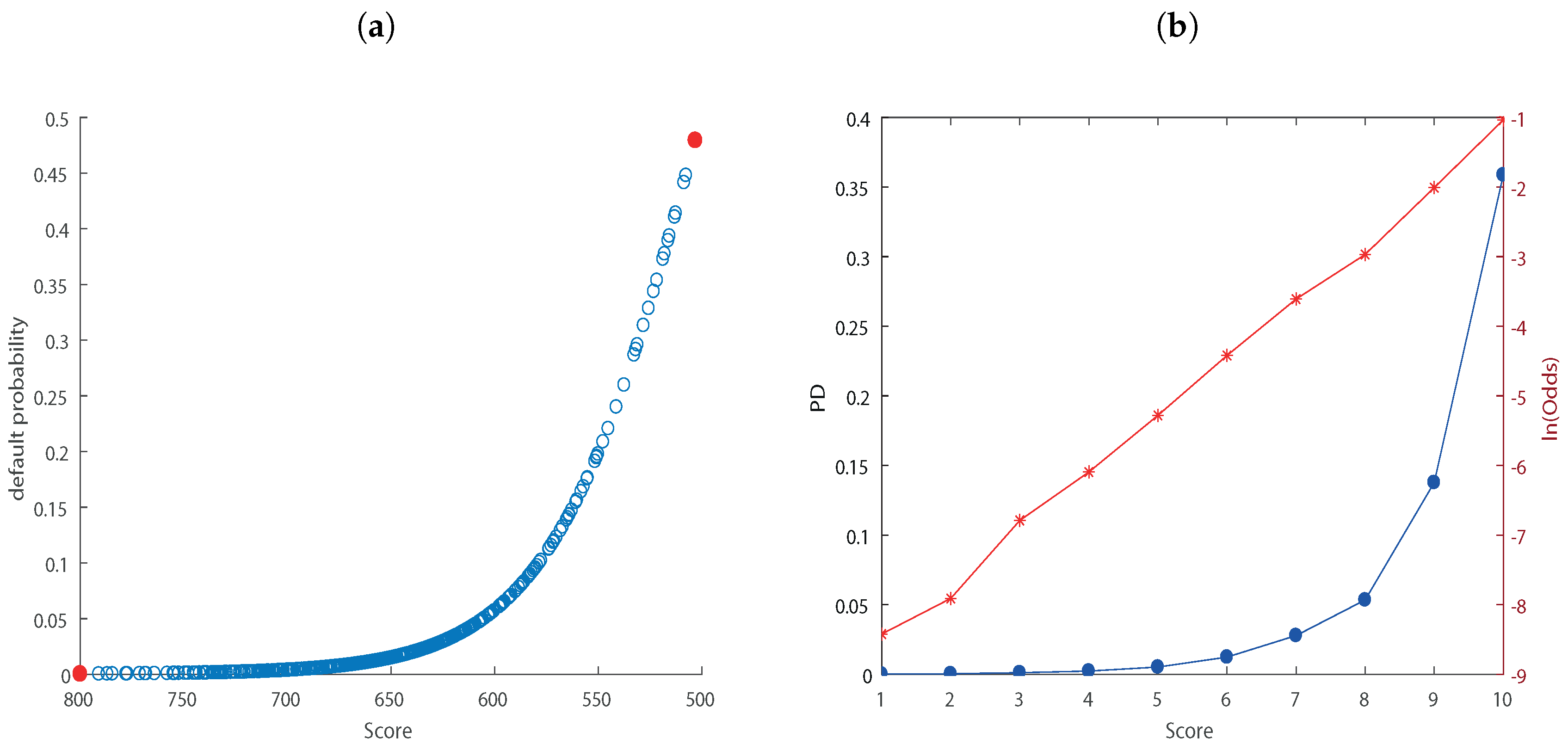
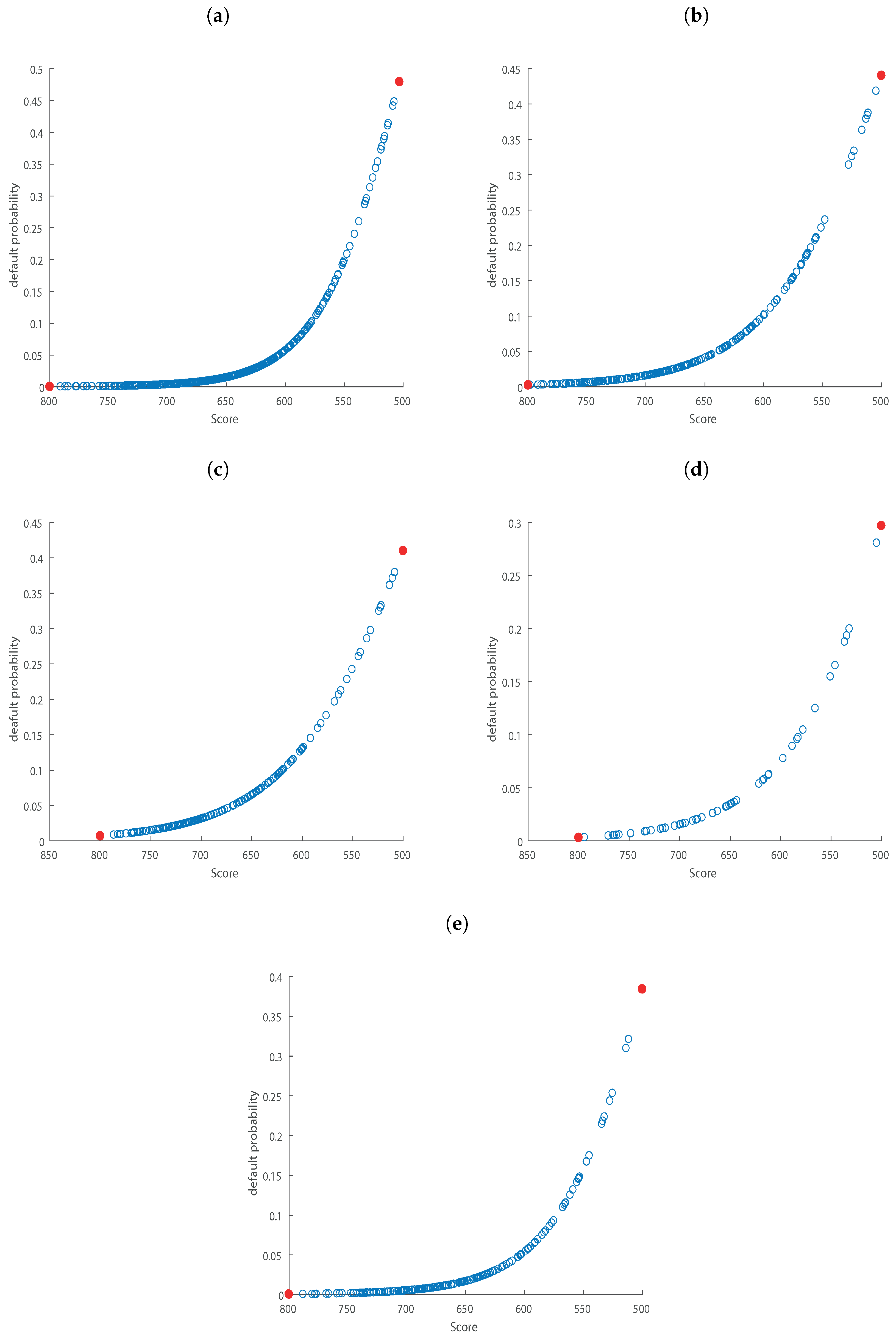
Figure 1a indicates the default probability associated with each score level for the first pool cut-off date. In the Appendix A we report the relationship for the other pool cut-off dates. We choose a score scale ranging from 500 (worst counterparties) to 800 points (best counterparties). We can see that as the score decreases, the associated default probability increases.
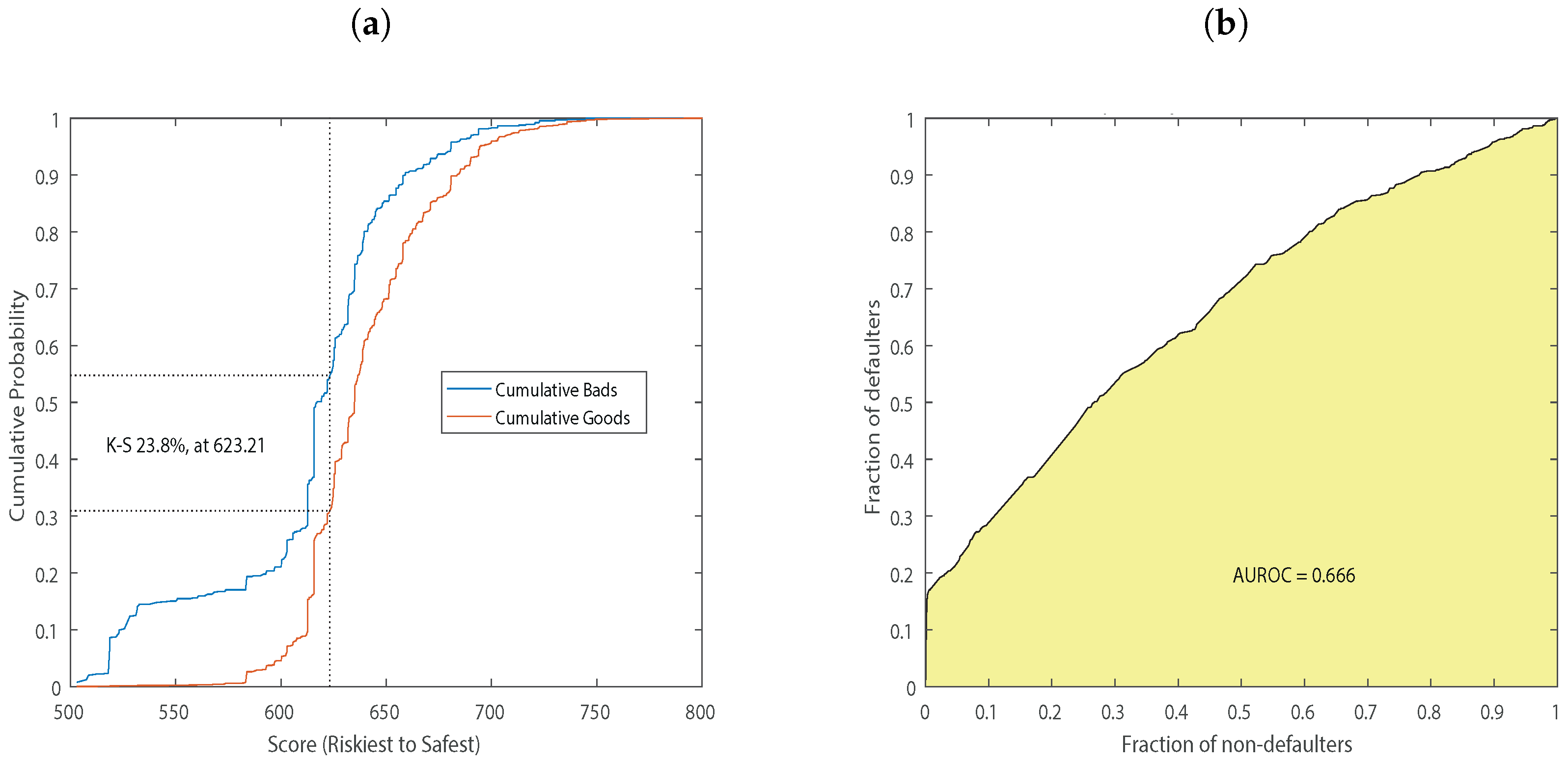
Validation statistics have the double purpose of measuring: (i) the power of the model, i.e., the ability to identify the dependence between the variables and the outputs produced and (ii) the divergence from the real results. We use Kolmogorov-Smirnov (KS) curve and Receiver Operating Characteristic (ROC) curve to measure model prediction capacity.
Kolmogorov-Smirnov (KS) The KS coefficient according to Mays and Lynas (2004) is the most widely used statistic within the United States for measuring the predictive power of rating systems. The Kolmogorov-Smirnov curve plots the cumulative distribution of non-defaulted and defaulted against the score, showing the percentage of non-defaulted and defaulted below a given score threshold, identifying it as the point of greatest divergence. According to Mays and Lynas (2004), KS values should be in the range 20%–70%. The goodness of the model should be highly questioned when values are below the lower bound. Value above the upper bound should be also considered with caution because they are ‘probably too good to be true’. The Kolmogorov-Smirnov statistic for a given cumulative distribution function is:
where is the supremum of the set of distances. The results on the dataset are included in Figure 2 and show values within the threshold for the first pool cut-off date. In the first report date with a 623 points score the KS value is . The statistics for the other pool cut-off dates are reported in Appendix A.
Lorenz curve and Gini coefficient In credit scoring, the Lorenz curve is used to analyze the model’s ability to distinguish between “good” (non-defaulted) and “bad” (defaulted), showing the cumulative percentage of defaulted and non-defaulted on the axes of the graph (Müller and Rönz 2000). When a model has no predictive capacity, there is perfect equality. The Gini Coefficient is widely used in Europe (Řezáč and Řezáč 2011), is derived from the Lorenz curve and calculates the area between the curve and diagonal in the Lorenz curve.
Gini coefficient The Gini coefficient is computed as:
where is the cumulative percentage of defaulters and is the cumulative percentage of non-defaulters. The result is a coefficient that measures the separation between the curve and the diagonal. Gini’s coefficient is a statistic used to understand how well the model can distinguish between “good” and “bad”.
This measure has the following limitations: (i) can be increased by increasing the range of indeterminates, i.e., who is neither “good” nor “bad” and (ii) is sensitive to the definition of the categories of variables both in terms of numbers and types. Operators’ experience, according to Anderson (2007), suggests that the level of the Gini coefficient should range between 30% and 50%, in order to have a satisfactory model.
Receiver Operating Characteristic (ROC) As reported by Satchel and Xia (2008), among the methodologies for assessing discriminatory power described in the literature the most popular one is the ROC curve and its summary index known as the area under the ROC (AUROC) curve. The ROC curve is created by plotting the true positive rate (TPR) against the false positive rate (FPR) at various threshold settings. The true-positive rate is also known as sensitivity and the false-positive rate is also known as the specificity. Specificity represents the ability to identify true negatives and can be calculated as 1 minus the specificity. The ROC therefore results from:
The curve is concave only when the relationship has a monotonous relationship with the event being studied. When the curve goes below the diagonal, the model is making a mistake in the prediction for both false positive and false negative but a reversal of the sign could correct it. This is very similar to the Gini coefficient, except that it represents the area under the ROC curve (AUROC), as opposed to measuring the part of the curve above it. The commonly used formula for the AUROC, as reported in (Anderson 2007, p. 207) is:
and shows that the area below the curve is equal to the probability that the score of a true positive (defaulted, ) is less than that of a true negative (non-defaulted, ), plus of the probability that the two scores are equal. A 50% value of AUROC implies that the model is making nothing more than a random guess. Table 6 shows the values of the statistics for the analyzed pool cut-off dates.
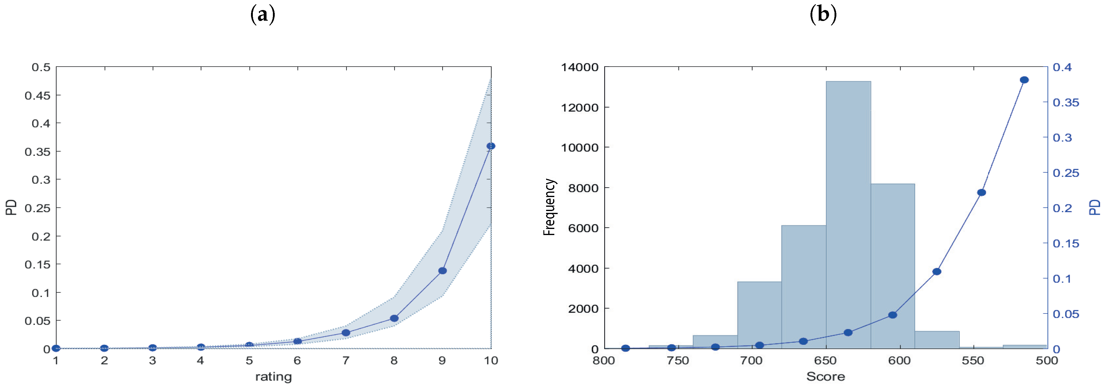
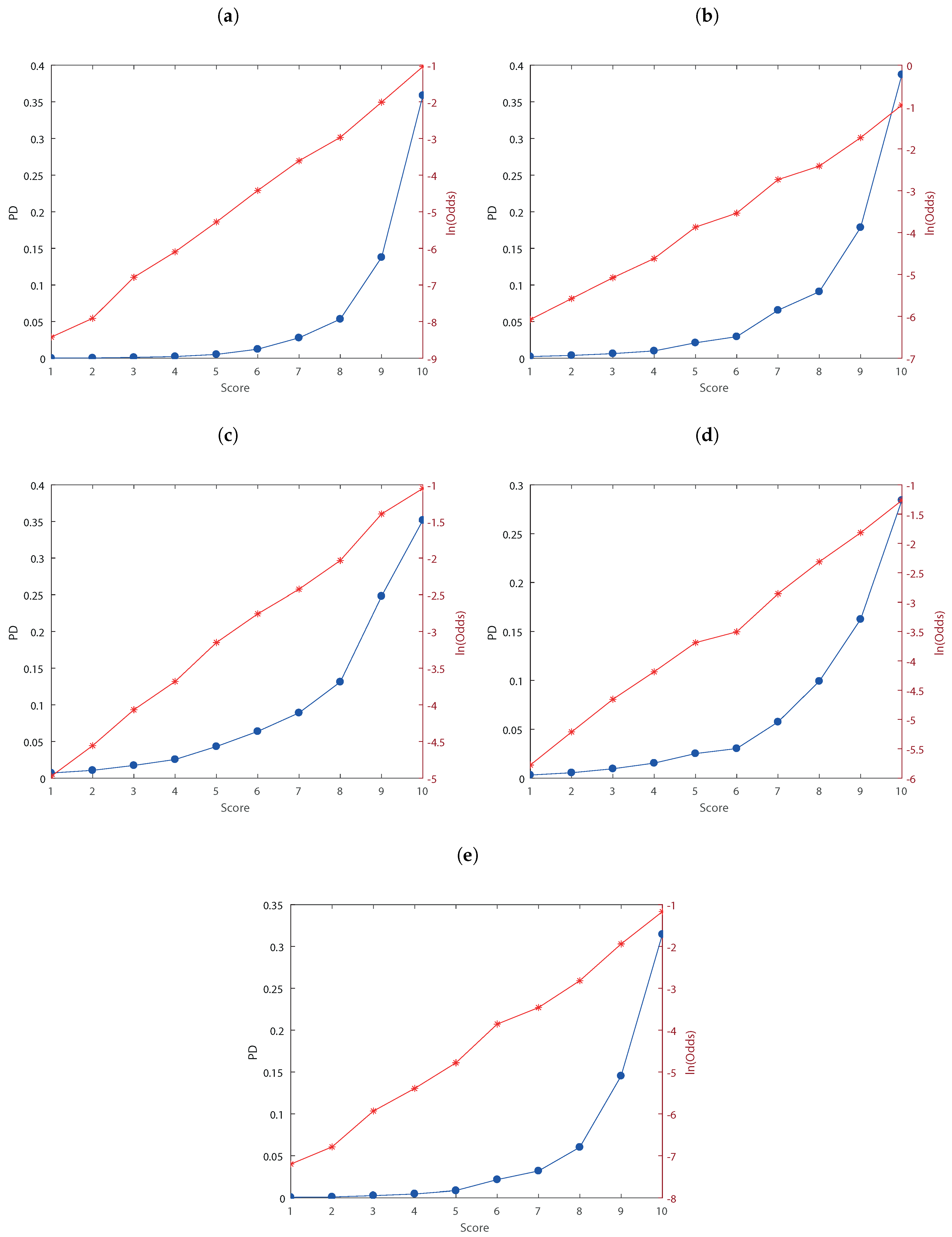
Once the predictive ability of the model is tested, it is possible to calculate the probability of default for classes of counterparties. In this respect, we create a master scale to associate a default probability to each score. As stated in Siddiqi (2017), a common approach is to have discrete scores scaled logarithmically. In our analysis, we set the target score to 500 with the odds doubling every 50 points which is commonly used in practice (Refaat 2011). The way to define the rating classes is through the creation of a cut-off defined with classes extension. Using the relationship between logarithm and exponential function it is possible to create the ranges for each rating class. The default probability vector by counterparty is linearized through the calculation of their natural logarithm, then this is divided into 10 equal classes and the logarithms of the cut-off of each class have been converted to identify the cut-off to be associated with each scoring class with an exponential function. With this procedure we calculate an average default probability for each range created (Figure 1b).
We validate the results obtained in the logistic regression with an out of sample analysis. In our analysis the validation has been performed by following directly Siddiqi (2017) which illustrated the standard procedure adopted in credit scoring. The industry norm is to use a random 70% (or 80%) of the development sample for building the model, while the remaining sample is kept for validation. When the scorecard is being developed on a small sample as in our case, it is preferred to use all the samples and validate the model on randomly selected samples of 50–80% length. Accordingly, we decided to use the second approach by selecting an out of sample of 50% of the total observations. We proceed as in the in-sample to analyze the statistics of separation and divergence for the out of sample, we report the statistics in Table 7. We observe that statistics do not differ substantially between the out of sample and the whole sample.
We carry out the analysis of the portfolio composition in all the pool cut-off dates analyzed. The revolving nature of the ABS may cause the composition of the portfolio under study to vary, even significantly. In general, the classes that include most of the counterparties are the central classes, as can be seen in Figure 3b. It is clear that the counterparties included in the ABS have an intermediate rating. For sake of completeness we report in Table 8 the actual default frequency in the sample per each rating class.
To estimate the recovery rate of a default exposure it is necessary to have information regarding the market value of the collateral, the administrative costs incurred for the credit recovery process and the cumulative recoveries. Since those data are not available in the dataset, we analyze the recovery rates starting directly from the data provided by the banks in the template under “AS37” with the name of “Bank internal Loss Given Default (LGD) estimate” which estimates the LGD of the exposure in normal economic conditions. The RR of the loan was calculated by applying the equation: .
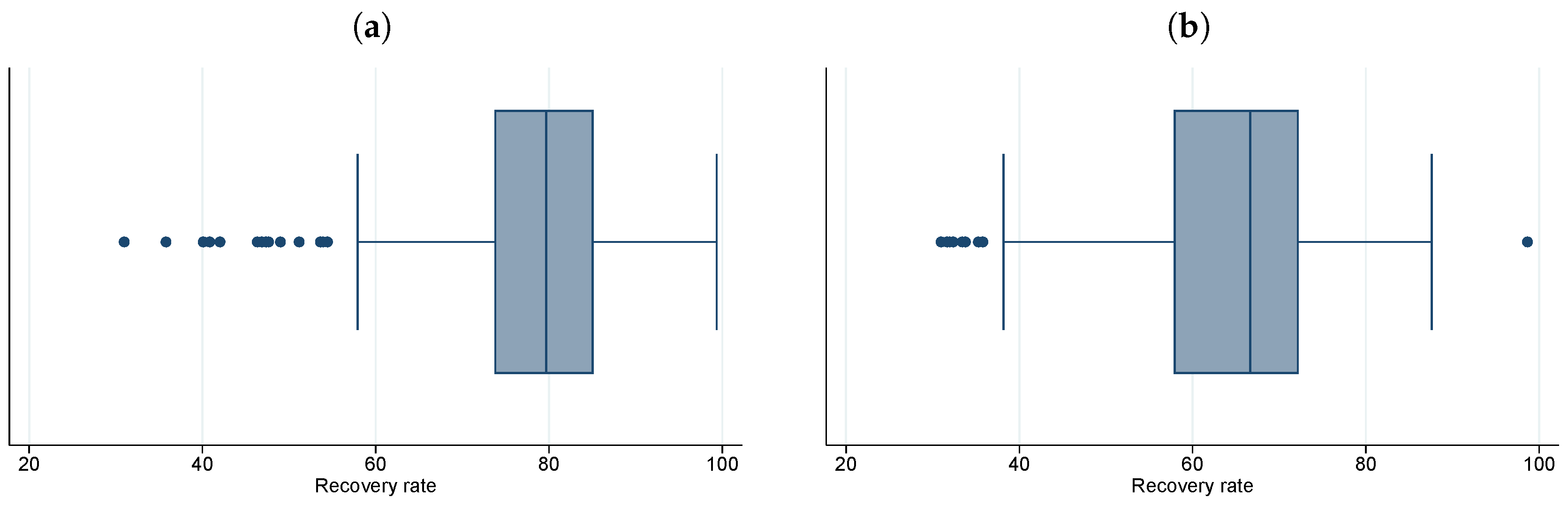
The average recovery rate through all the collaterals related to one loan calculated by the bank is different depending on the level of protection offered, as evidenced by Figure 4.
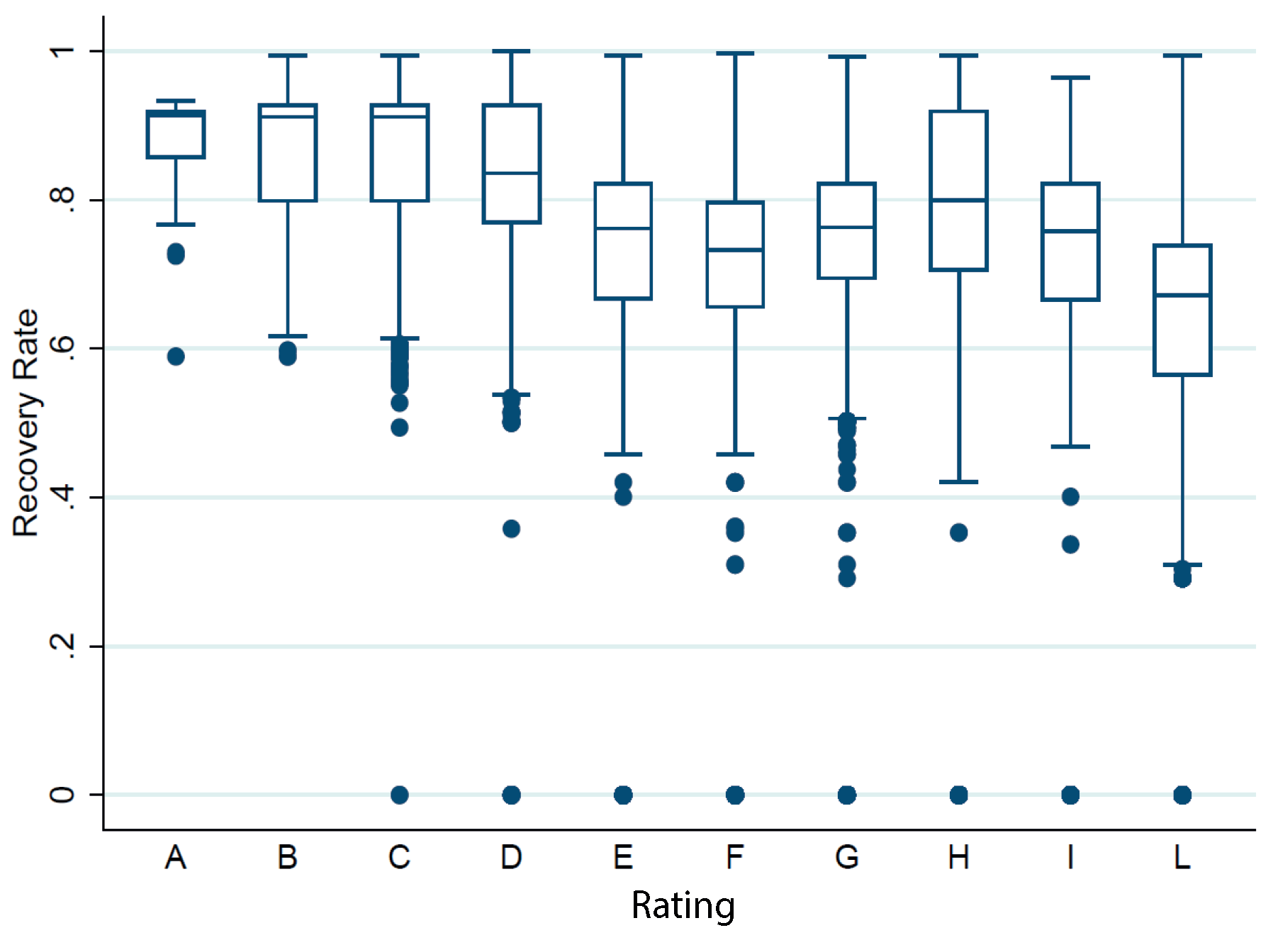
As can be seen in Figure 4, the originator estimates a lower recovery rate for unsecured exposures than for secured loans. The average RR for secured exposures is , while for unsecured exposures on average the bank expects to recover of the amount granted. Figure 5 and Table 9 show the recovery rate calculated by the bank by rating level, it can be seen that the average recovery rate calculated by the bank tends to decrease as the counterparty’s rating deteriorates, even if not monotonously.
To investigate portfolio loss distribution we implement CREDITRISK+™ model on a representative sample of approximately 20,000 counterparties, of which 10,000 refer to loans terminated (repaid or defaulted) before the first pool cut-off date while the remaining 10,000 are active at the latest pool cut-off dates and are used to provide a forecast of the future loss profile of the portfolio.
CREDITRISK+™ can be applied to different types of credit exposure including corporate and retail loans, derivatives and traded bonds. In our analysis we implement it on a portfolio of SMEs credit exposures. It is based on a portfolio approach to modelling credit risk that makes no assumption about the causes of default, this approach is similar to the one used in market risk, where no assumptions are made about causes of market price movements. CREDITRISK+™ considers default rates as continuous random variables and incorporates the volatility of default rates to capture default rates level uncertainty. The data used in the model are: (i) credit exposures; (ii) borrower default rates; (iii) borrower default rate volatilities and (iv) recovery rates. In order to reduce the computational difficulties, the exposures are adjusted by anticipated recovery rates in order to calculate the loss in case of default event. We consider recovery rates provided by ED and include them in the database. The exposures, net of recovery rates, are divided into bands with similar exposures. The model assumes that each exposure has a definite known default probability over a specific time horizon. Thus
We introduce the probability generating function (PGF) defined in terms of an auxiliary variable z
An individual borrower either defaults or does not default, therefore the probability generating function for a single borrower is6:
CREDITRISK+™ assumes that default events are independent, hence, the probability generating function for the whole portfolio is the product of the individual PGF, as shown in Equation (17)
and could be written as:
The Credit Risk Plus model CSFB (1997) assumes that a borrower’s default probabilities are uniformly small, therefore powers of those probabilities can be ignored and the logarithm can be replaced using the expression7
and, in the limit, Equation (18) becomes
where
represents the expected number of default events in one year from the whole portfolio. is expanded in its Taylor series in order to identify the distribution corresponding to this PGF:
thus considering small individual default probabilities from Equation (22) the probability of realising n default events in the portfolio in one year is given by:
where we obtain the Poisson distribution for the distribution of the number of defaults. The distribution has only one parameter, the expected number of defaults . The distribution does not depend on the number of exposures in the portfolio or the individual probabilities of default provided that they are uniformly small. Real portfolio loss differs from the Poisson distribution, historical evidence shows in fact that the standard deviation of default event frequencies is much larger than , the standard deviation of the Poisson distribution with mean . We can espress the expected loss in terms of the probability of default events
where
is the common exposure in the exposure band, is the expected loss in the exposure band and is the expected number of defaults in the exposure band. We can derive the distribution of default losses as with as the PGF for losses expressed in multiples of an unit of exposure L
The inputs that we include are therefore the average of the estimate of the probability of default calculated through the logistic regression and the relative volatility calculated through the pool cut-off dates. The exposure included in the model was calculated net of the recovery rates estimated by the bank. As stated previously, since the data to obtain the recovery rate are not available, we test the model with bank own recovery rates estimates. The mean and volatility values of the default probabilities are shown in Table 10. For the sake of completeness, we have also reported the mean and standard deviation of the default frequencies.
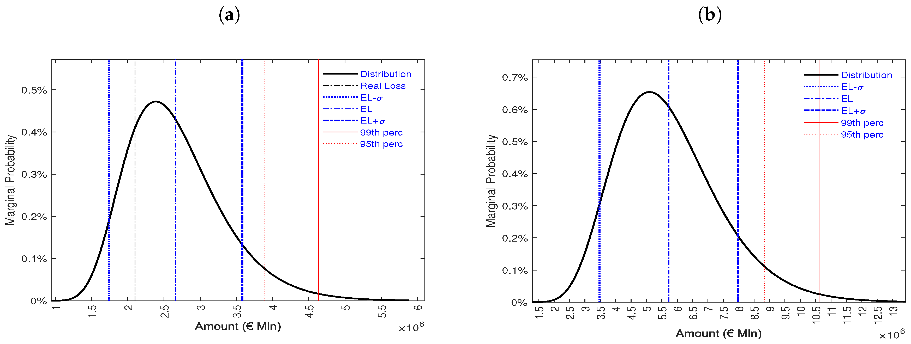
The model’s estimate on the historical data of the loans terminated in the first available pool cut-off date provides an indication of the expected loss of 2,661,592 Euro against a total exposure of million Euro with a standard deviation of 670,422 Euro (Table 11).
The real loss of the analysed portfolio calculated on all terminated loans is 2.10 million euro, lower than the expected loss computed by the model but within the threshold. The estimated expected loss by the model is of the capital exposed to risk which represents the outstanding amount net of recovery rates.
The analysis shows that the portfolio before the first pool cut-off date lost a total of of its value against an estimated loss of . Even though the model with the input data used overestimates the expected loss, it is in the range. Due to the small number of counterparts and the lack of homogeneity of the data, an estimation error is possible. With a view to analyzing future performance, only loans active in the last pool cut-off date are kept in the portfolio and estimates of PD and volatility have been used as an approximation of the probability of future default. In a sample of 10,000 current counterparties in last pool cut-off date the capital exposed to the total risk of loss is 247 million with an expected loss of million corresponding to of the total (Table 12). This means that after the last available report the portfolio would have lost an additional of the capital exposed to risk before the withdrawal.
The average loss in the sample is while the estimate of the future loss in the pool cut-off dates is a further . Panel Figure 6a shows the loss distribution for terminated loans and Panel Figure 6b illustrates the loss distribution for active exposures.
In accordance with the studies conducted by CRIF8, Italian company specialized in credit bureau and business information, the default rates of Italian SMEs are around 6%, above those calculated in the analyzed sample. Assuming that recovery rates are similar to those of companies not included in the portfolio of securitized exposures, we can assume that the loss profiles for securitized portfolios are less severe than for exposures retained in the bank’s balance sheet and not securitized.
4. Conclusions
Small and medium enterprises play a main role in the European Union in terms of jobs and added value in the real economy. These enterprises are largely reliant on bank-related lending channels and do not have easy access to alternative channels such as the securitisation mechanism.
In this paper, we investigated the default probability, recovery rates and loss distribution of a portfolio of securitised loans granted to Italian small and medium enterprises. SMEs have a share in Italy that is larger than the average of the European Union and thus represent an interesting market to be investigated. We make use of loan level data information provided by the European DataWarehouse and employ a logistic regression to estimate their default probability.
The aim of our analysis focused on the comparison of the riskiness of securitised loans with the average of bank lending in the SME market. We collected the SME’s exposures from the European DataWarehouse and exploited the informational content of the variables to compute a credit score to estimate the probability of default at a firm level.
Our results indicate that the default rates for securitised loans are lower than the average bank lending for the Italian SMEs’ exposures as shown in Caprara et al. (2015). The investigation should be extended to the European level in order to compare the different SME markets using the same timeframe as in the proposed Italian analysis. We leave these aspects for future research.
Author Contributions
The authors have contributed jointly to all of the sections of the paper.
Funding
This research received no external funding.
Acknowledgments
We thank three anonymous Reviewers and Editors for their insightful comments and suggestions.
Conflicts of Interest
The authors declare no conflict of interest.
Appendix A
Equation (A1) reports the regression output for all the analyzed pool cut-off dates. Figure A1 illustrates the relationship between Score and default probability, Figure A2 shows the masterscale and Figure A3 shows masterscale and borrower distribution. Table A1 reports portfolio composition per rating class, Table A2 shows default frequencies in the sample and Table A3 compares default probabilities estimated by regression model and default frequencies in the sample.
Figure A1.
The figure illustrates the relationship between Score (x-axis) and default probability (y-axis) for 2014H1 (Panel (a)), 2014H2 (Panel (b)), 2015H1 (Panel (c)), 2015H2 (Panel (d)), 2016H1 (Panel (e)).
Figure A1.
The figure illustrates the relationship between Score (x-axis) and default probability (y-axis) for 2014H1 (Panel (a)), 2014H2 (Panel (b)), 2015H1 (Panel (c)), 2015H2 (Panel (d)), 2016H1 (Panel (e)).

Figure A2.
Master scale for the sample. We illustrate 2014H1 (Panel (a)), 2014H2 (Panel (b)), 2015H1 (Panel (c)), 2015H2 (Panel (d)), 2016H1 (Panel (e)).
Figure A2.
Master scale for the sample. We illustrate 2014H1 (Panel (a)), 2014H2 (Panel (b)), 2015H1 (Panel (c)), 2015H2 (Panel (d)), 2016H1 (Panel (e)).

Figure A3.
Master scale and borrower distribution for 2014H1(Panel (a,b)), 2014H2 (Panel (c,d)), 2015H1 (Panel (e,f)), 2015H2 (Panel (g,h)), 2016H1 (Panel (i,j)).
Figure A3.
Master scale and borrower distribution for 2014H1(Panel (a,b)), 2014H2 (Panel (c,d)), 2015H1 (Panel (e,f)), 2015H2 (Panel (g,h)), 2016H1 (Panel (i,j)).


Table A1.
The table shows the portfolio composition per rating across the pool cut-off dates. The distribution of counterparties is mainly concentrated in the intermediate rating classes.
Table A1.
The table shows the portfolio composition per rating across the pool cut-off dates. The distribution of counterparties is mainly concentrated in the intermediate rating classes.
| 2014H1 | 2014H2 | 2015H1 | 2015H2 | 2016H1 | |||||||||||||||
|---|---|---|---|---|---|---|---|---|---|---|---|---|---|---|---|---|---|---|---|
| Rating | Freq. | Perc. | Cum. | Rating | Freq. | Perc. | Cum. | Rating | Freq. | Perc. | Cum. | Rating | Freq. | Perc. | Cum. | Rating | Freq. | Perc. | Cum. |
| A | 4 | 0.01 | 0.01 | A | 31 | 0.11 | 0.11 | A | 57 | 0.25 | 0.25 | A | 106 | 0.81 | 0.81 | A | 42 | 0.41 | 0.41 |
| B | 30 | 0.09 | 0.10 | B | 1250 | 4.52 | 4.63 | B | 1919 | 8.57 | 8.82 | B | 1306 | 10.03 | 10.84 | B | 95 | 0.92 | 1.33 |
| C | 301 | 0.92 | 1.02 | C | 2519 | 9.11 | 13.74 | C | 8002 | 35.72 | 44.54 | C | 1506 | 11.56 | 22.41 | C | 523 | 5.06 | 6.39 |
| D | 716 | 2.18 | 3.20 | D | 1288 | 4.66 | 18.39 | D | 7610 | 33.97 | 78.51 | D | 502 | 3.85 | 26.26 | D | 1562 | 15.12 | 21.50 |
| E | 3498 | 10.65 | 13.85 | E | 7355 | 26.59 | 44.98 | E | 1775 | 7.92 | 86.43 | E | 1413 | 10.85 | 37.11 | E | 1149 | 11.12 | 32.62 |
| F | 7272 | 22.15 | 36.00 | F | 12165 | 43.97 | 88.95 | F | 2060 | 9.20 | 95.63 | F | 6877 | 52.81 | 89.92 | F | 2988 | 28.92 | 61.54 |
| G | 15679 | 47.75 | 83.75 | G | 2660 | 9.62 | 98.57 | G | 751 | 3.35 | 98.98 | G | 1163 | 8.93 | 98.85 | G | 3148 | 30.47 | 92.01 |
| H | 4984 | 15.18 | 98.93 | H | 150 | 0.54 | 99.11 | H | 72 | 0.32 | 99.30 | H | 30 | 0.23 | 99.08 | H | 711 | 6.88 | 98.89 |
| I | 153 | 0.47 | 99.40 | I | 82 | 0.30 | 99.41 | I | 115 | 0.51 | 99.81 | I | 39 | 0.30 | 99.38 | I | 32 | 0.31 | 99.20 |
| L | 197 | 0.60 | 100.00 | L | 164 | 0.59 | 100.00 | L | 42 | 0.19 | 100.00 | L | 81 | 0.62 | 100.00 | L | 83 | 0.80 | 100.00 |
Table A2.
The table shows rating (column 1), amount of non-defaulted loans (column 2), amount of defaulted (column 3), default frequency (column 4) and total number of loans included in the sample per rating class (column 5). We report the statistics for the different pool cut-off dates.
Table A2.
The table shows rating (column 1), amount of non-defaulted loans (column 2), amount of defaulted (column 3), default frequency (column 4) and total number of loans included in the sample per rating class (column 5). We report the statistics for the different pool cut-off dates.
| 2014H1 | Non-Defaulted | Defaulted | pd_actual (%) | Total | 2014H2 | Non-Defaulted | Defaulted | pd_actual (%) | Total | |
|---|---|---|---|---|---|---|---|---|---|---|
| A | 4 | 0 | 0.00 | 4 | 31 | 0 | 0.00 | 31 | ||
| B | 30 | 0 | 0.00 | 30 | 1229 | 21 | 1.68 | 1250 | ||
| C | 298 | 3 | 1.00 | 301 | 2482 | 37 | 1.47 | 2519 | ||
| D | 707 | 9 | 1.26 | 716 | 1267 | 21 | 1.63 | 1288 | ||
| E | 3452 | 46 | 1.32 | 3498 | 7186 | 169 | 2.30 | 7355 | ||
| F | 7169 | 103 | 1.42 | 7272 | 11819 | 346 | 2.84 | 12165 | ||
| G | 15264 | 415 | 2.65 | 15679 | 2587 | 73 | 2.74 | 2660 | ||
| H | 4810 | 174 | 3.49 | 4984 | 146 | 4 | 2.67 | 150 | ||
| I | 134 | 19 | 12.42 | 153 | 58 | 24 | 29.27 | 82 | ||
| L | 62 | 135 | 68.53 | 197 | 46 | 118 | 71.95 | 164 | ||
| 2015H1 | Non-Defaulted | Defaulted | pd_actual (%) | Total | 2015H2 | Non-Defaulted | Defaulted | pd_actual (%) | Total | |
| A | 57 | 0 | 0.00 | 57 | 105 | 1 | 0.94 | 106 | ||
| B | 1890 | 29 | 1.51 | 1919 | 1286 | 20 | 1.53 | 1306 | ||
| C | 7825 | 177 | 2.21 | 8002 | 1478 | 28 | 1.86 | 1506 | ||
| D | 7366 | 244 | 3.21 | 7610 | 491 | 11 | 2.19 | 502 | ||
| E | 1742 | 33 | 1.86 | 1775 | 1377 | 36 | 2.55 | 1413 | ||
| F | 2015 | 45 | 2.18 | 2060 | 6681 | 196 | 2.85 | 6877 | ||
| G | 715 | 36 | 4.79 | 751 | 1142 | 21 | 1.81 | 1163 | ||
| H | 69 | 3 | 4.17 | 72 | 30 | 0 | 0.00 | 30 | ||
| I | 37 | 78 | 67.83 | 115 | 36 | 3 | 7.69 | 39 | ||
| L | 8 | 34 | 80.95 | 42 | 25 | 56 | 69.14 | 81 | ||
| 2016H1 | Non-Defaulted | Defaulted | pd_actual % | Total | ||||||
| A | 42 | 0 | 0.00 | 42 | ||||||
| B | 95 | 0 | 0.00 | 95 | ||||||
| C | 517 | 6 | 1.15 | 523 | ||||||
| D | 1547 | 15 | 0.96 | 1562 | ||||||
| E | 1136 | 13 | 1.13 | 1149 | ||||||
| F | 2929 | 59 | 1.97 | 2988 | ||||||
| G | 3050 | 98 | 3.11 | 3148 | ||||||
| H | 695 | 16 | 2.25 | 711 | ||||||
| I | 27 | 5 | 15.63 | 32 | ||||||
| L | 38 | 45 | 54.22 | 83 |
Table A3.
The table compares default probabilities estimated by the regression model (pd_model) and default frequencies (pd_actual) across the pool cut-off dates. The values of the two statistics are close, especially for the intermediate rating classes.
Table A3.
The table compares default probabilities estimated by the regression model (pd_model) and default frequencies (pd_actual) across the pool cut-off dates. The values of the two statistics are close, especially for the intermediate rating classes.
| 2014H1 | 2014H2 | 2015H1 | 2015H2 | 2016H1 | ||||||||||
|---|---|---|---|---|---|---|---|---|---|---|---|---|---|---|
| pd_model | pd_actual | pd_model | pd_actual | pd_model | pd_actual | pd_model | pd_actual | pd_model | pd_actual | |||||
| A | 0.02 | 0.00 | 0.23 | 0.00 | 0.69 | 0.00 | 0.31 | 0.94 | 0.08 | 0.00 | ||||
| B | 0.04 | 0.00 | 0.38 | 1.68 | 1.05 | 1.51 | 0.55 | 1.53 | 0.11 | 0.00 | ||||
| C | 0.11 | 1.00 | 0.63 | 1.47 | 1.72 | 2.21 | 0.95 | 1.86 | 0.27 | 1.15 | ||||
| D | 0.23 | 1.26 | 1.00 | 1.63 | 2.54 | 3.21 | 1.53 | 2.19 | 0.46 | 0.96 | ||||
| E | 0.52 | 1.32 | 2.11 | 2.30 | 4.31 | 1.86 | 2.51 | 2.55 | 0.86 | 1.13 | ||||
| F | 1.23 | 1.42 | 2.95 | 2.84 | 6.37 | 2.18 | 3.02 | 2.85 | 2.15 | 1.97 | ||||
| G | 2.78 | 2.65 | 6.55 | 2.74 | 8.90 | 4.79 | 5.74 | 1.81 | 3.19 | 3.11 | ||||
| H | 5.34 | 3.49 | 9.09 | 2.67 | 13.12 | 4.17 | 9.92 | 0.00 | 6.02 | 2.25 | ||||
| I | 13.77 | 12.42 | 17.85 | 29.27 | 24.81 | 67.83 | 16.26 | 7.69 | 14.54 | 15.63 | ||||
| L | 35.87 | 68.53 | 38.72 | 71.95 | 35.17 | 80.95 | 28.42 | 69.14 | 31.45 | 54.22 | ||||
References
- Altman, Edward I. 1968. Financial ratios, discriminant analysis and the prediction of corporate bankruptcy. The Journal of Finance 23: 589–609. [Google Scholar] [CrossRef]
- Altman, Edward I. 1977. Predicting performance in the savings and loan association industry. Journal of Monetary Economics 3: 443–66. [Google Scholar] [CrossRef]
- Anderson, Raymond. 2007. The Credit Scoring Toolkit: Theory and Practice for Retail Credit Risk Management and Decision Automation. Oxford: Oxford University Press. [Google Scholar]
- Barnes, Paul. 1982. Methodological implications of non-normally distributed financial ratios. Journal of Business Finance & Accounting 9: 51–62. [Google Scholar]
- Beaver, William H. 1968. Alternative accounting measures as predictors of failure. The Accounting Review 43: 113–22. [Google Scholar]
- Blum, Marc. 1974. Failing company discriminant analysis. Journal of Accounting Research 12: 1–25. [Google Scholar] [CrossRef]
- Bryant, Stephanie M. 1997. A case-based reasoning approach to bankruptcy prediction modeling. Intelligent Systems in Accounting, Finance & Management 6: 195–214. [Google Scholar]
- Buta, Paul. 1994. Mining for financial knowledge with cbr. Ai Expert 9: 34–41. [Google Scholar]
- Caprara, Cristina, Davide Tommaso, and Roberta Mantovani. 2015. Corporate Credit Risk Research. Technical Report. Bologna: CRIF Rating. [Google Scholar]
- Chesser, Delton L. 1974. Predicting loan noncompliance. The Journal of Commercial Bank Lending 56: 28–38. [Google Scholar]
- Cortes, Corinna, and Vladimir Vapnik. 1995. Support-vector networks. Machine Learning 20: 273–97. [Google Scholar] [CrossRef]
- CSFB. 1997. Credit Risk+. Technical Document. New York: Credit Suisse First Boston. [Google Scholar]
- Deakin, Edward B. 1972. A discriminant analysis of predictors of business failure. Journal of Accounting Research 10: 167–79. [Google Scholar] [CrossRef]
- Dietsch, Michel, Klaus Düllmann, Henri Fraisse, Philipp Koziol, and Christine Ott. 2016. Support for the Sme Supporting Factor: Multi-Country Empirical Evidence on Systematic Risk Factor for Sme Loans. Frankfurt am Main: Deutsche Bundesbank Discussion Paper Series. [Google Scholar]
- Edmister, Robert O. 1972. An empirical test of financial ratio analysis for small business failure prediction. Journal of Financial and Quantitative Analysis 7: 1477–93. [Google Scholar] [CrossRef]
- European Parliament, Council of the European Union. 2013. Regulation (EU) No 575/2013 on Prudential Requirements for Credit Institutions and Investment Firms and Amending Regulation (EU) No 648/2012. Brussels: Official Journal of the European Union. [Google Scholar]
- Hamer, Michelle M. 1983. Failure prediction: Sensitivity of classification accuracy to alternative statistical methods and variable sets. Journal of Accounting and Public Policy 2: 289–307. [Google Scholar] [CrossRef]
- Hand, David J., and William E. Henley. 1997. Statistical classification methods in consumer credit scoring: A review. Journal of the Royal Statistical Society: Series A (Statistics in Society) 160: 523–41. [Google Scholar] [CrossRef]
- Hopkin, Richard, Anna Bak, and Sidika Ulker. 2014. High-Quality Securitization for Europe—The Market at a Crossroads. London: Association for Financial Markets in Europe. [Google Scholar]
- Jo, Hongkyu, Ingoo Han, and Hoonyoung Lee. 1997. Bankruptcy prediction using case-based reasoning, neural networks, and discriminant analysis. Expert Systems with Applications 13: 97–108. [Google Scholar] [CrossRef]
- Karels, Gordon V., and Arun J. Prakash. 1987. Multivariate normality and forecasting of business bankruptcy. Journal of Business Finance & Accounting 14: 573–93. [Google Scholar]
- Kim, Hong Sik, and So Young Sohn. 2010. Support vector machines for default prediction of smes based on technology credit. European Journal of Operational Research 201: 838–46. [Google Scholar] [CrossRef]
- Martin, Daniel. 1977. Early warning of bank failure: A logit regression approach. Journal of Banking & Finance 1: 249–76. [Google Scholar]
- Mays, Elizabeth, and Niall Lynas. 2004. Credit Scoring for Risk Managers: The Handbook for Lenders. Mason: Thomson/South-Western Ohio. [Google Scholar]
- Min, Jae H., and Young-Chan Lee. 2005. Bankruptcy prediction using support vector machine with optimal choice of kernel function parameters. Expert Systems With Applications 28: 603–14. [Google Scholar] [CrossRef]
- Mironchyk, Pavel, and Viktor Tchistiakov. 2017. Monotone Optimal Binning Algorithm for Credit Risk Modeling. Utrecht: Working Paper. [Google Scholar]
- Müller, Marlene, and Bernd Rönz. 2000. Credit scoring using semiparametric methods. In Measuring Risk in Complex Stochastic Systems. Berlin and Heidelberg: Springer, pp. 83–97. [Google Scholar]
- Odom, Marcus D., and Ramesh Sharda. 1990. A neural network model for bankruptcy prediction. Paper Presented at 1990 IJCNN International Joint Conference on Neural Networks, San Diego, CA, USA, June 17–21; pp. 163–68. [Google Scholar]
- Ohlson, James A. 1980. Financial ratios and the probabilistic prediction of bankruptcy. Journal of Accounting Research 18: 109–31. [Google Scholar] [CrossRef]
- Park, Cheol-Soo, and Ingoo Han. 2002. A case-based reasoning with the feature weights derived by analytic hierarchy process for bankruptcy prediction. Expert Systems with Applications 23: 255–64. [Google Scholar] [CrossRef]
- Refaat, Mamdouh. 2011. Credit Risk Scorecard: Development and Implementation Using SAS. Available online: Lulu.com (accessed on 15 October 2018).
- Řezáč, Martin, and František Řezáč. 2011. How to measure the quality of credit scoring models. Finance a úvěr: Czech Journal of Economics and Finance 61: 486–507. [Google Scholar]
- Satchel, Stephen, and Wei Xia. 2008. Analytic models of the roc curve: Applications to credit rating model validation. In The Analytics of Risk Model Validation. Amsterdam: Elsevier, pp. 113–33. [Google Scholar]
- Siddiqi, Naeem. 2017. Intelligent Credit Scoring: Building and Implementing Better Credit Risk Scorecards. Hoboken: John Wiley & Sons. [Google Scholar]
- Sinkey, Jr., and Joseph F. 1975. A multivariate statistical analysis of the characteristics of problem banks. The Journal of Finance 30: 21–36. [Google Scholar] [CrossRef]
- Stuhr, David P., and Robert Van Wicklen. 1974. Rating the financial condition of banks: A statistical approach to aid bank supervision. Monthly Review 56: 233–38. [Google Scholar]
- Tam, Kar Yan, and Melody Y. Kiang. 1992. Managerial applications of neural networks: The case of bank failure predictions. Management Science 38: 926–47. [Google Scholar] [CrossRef]
- Thomas, Lyn C., Dabid B. Edelman, and Jonathan N. Crook. 2002. Credit Scoring and Its Applications: Siam Monographs on Mathematical Modeling and Computation. Philadelphia: University City Science Center, SIAM. [Google Scholar]
- Van Gestel, Tony, Bart Baesens, Johan Suykens, Marcelo Espinoza, Dirk-Emma Baestaens, Jan Vanthienen, and Bart De Moor. 2003. Bankruptcy prediction with least squares support vector machine classifiers. Paper presented at 2003 IEEE International Conference on Computational Intelligence for Financial Engineering, Hong Kong, March 20–23; pp. 1–8. [Google Scholar]
- Wilson, Rick L., and Ramesh Sharda. 1994. Bankruptcy prediction using neural networks. Decision Support Systems 11: 545–57. [Google Scholar] [CrossRef]
- Zeng, Guoping. 2013. Metric divergence measures and information value in credit scoring. Journal of Mathematics 2013: 848271. [Google Scholar] [CrossRef]
- Zhang, Guoqiang, Michael Y. Hu, B. Eddy Patuwo, and Daniel C. Indro. 1999. Artificial neural networks in bankruptcy prediction: General framework and cross-validation analysis. European Journal of Operational Research 116: 16–32. [Google Scholar] [CrossRef] [Green Version]
| 1. | The list of the ECB templates is available at https://www.ecb.europa.eu/paym/coll/loanlevel/transmission/html/index.en.html. |
| 2. | The ECB and the national central banks of the Eurosystem have been lending unlimited amounts of capital to the bank system as a response to the financial crisis. For more information see: https://www.ecb.europa.eu/explainers/tell-me-more/html/excess_liquidity.en.html. |
| 3. | A default shall be considered to have occurred with regard to a particular obligor when either or both of the following have taken place: (a) the institution considers that the obligor is unlikely to pay its credit obligations to the institution, the parent undertaking or any of its subsidiaries in full, without recourse by the institution to actions such as realising security; (b) the obligor is past due more than 90 days on any material credit obligation to the institution, the parent undertaking or any of its subsidiaries. Relevant authorities may replace the 90 days with 180 days for exposures secured by residential or SME commercial real estate in the retail exposure class (as well as exposures to public sector entities). |
| 4. | CRIF Ratings is an Italian credit rating agency authorized to assign ratings to non-financial companies based in the European Union. The agency is subject to supervision by the ESMA (European Securities and Markets Authority) and has been recognized as an ECAI (External Credit Assessment Institution). |
| 5. | The complete list of fields definitions and criteria can be found at https://www.ecb.europa.eu/paym/coll/loanlevel/shared/files/RMBS_Taxonomy.zip?bc2bf6081ec990e724c34c634cf36f20. |
| 6. | The Credit Risk Plus model assumes independence between default events. Therefore, the probability generating function for the whole portfolio corresponds to the product of the individual probability generating functions. |
| 7. | The approximation ignores terms of degree 2 and higher in the default probabilities. The expression derived from this approximation is exact in the limit as the PD tends to zero, and five good approximations in practice. |
| 8. |
Figure 1.
Panel (a) illustrates the relationship between score and PD. For each company we compute a score based on the logistic regression output that is an indication of individual PD. Panel (b) shows the master scale. This is an indicator of the counterparty’s riskiness level. For its creation, we follow the approach presented by Siddiqi (2017). The default probability is linearized through the calculation of the natural logarithm, then the vector of the logarithms of the PD is divided into 10 equal-sized classes and the logarithms of the cut-offs of each class is converted to identify the cut-offs to be associated with each scoring class with an exponential function.

Figure 2.
Panel (a) illustrates the Kolmogorov-Smirnov curve and the associated statistics for the first pool cut-off date. We show that the KS statistic associated to a score of is . Panel (b) reports the ROC curve and the AUROC value for the first report date. Table 6 reports AUROC, KS statistic and KS score for the entire sample.

Figure 3.
Panel (a) reports the final master scale obtained for the first pool cut-off date. To create the master scale we linearize the PD vector through the calculation of the natural logarithm, then this is divided into 10 equal classes and we convert the log of the cut-off of each class in order to identify the cut-off to be associated with each score with the exponential function. Panel (b) confirms the frequency of borrowers for each class. In the right y-axis we indicate the default probability associated for each class and in the left y-axis is indicated the frequency of the loans.

Figure 4.
Considering the variable Seniority (field AS26 in the ECB template) we divide secured from unsecured loans. Panel (a) reports the box plot for the secured loans included in the total sample (taking into account all the pool cut-off dates), Panel (b) shows the box plot for unsecured loans. It is clear that banks expect to recover more from secured loans compared to unsecured ones.

Figure 5.
The Figure shows the box plot of the recovery rates computed by the banks divided into the rating classes. We note that the RR decreases from A to L, even though not monotonously.
Figure 5.
The Figure shows the box plot of the recovery rates computed by the banks divided into the rating classes. We note that the RR decreases from A to L, even though not monotonously.

Figure 6.
The figure illustrates the loss distribution for unactive loans at the pool cut-off date 2014H1 (Panel (a)) and for active loans at the report date 2016H1 (Panel (b)). We indicate in the figure loss distribution (black solid line), real loss portfolio loss (black dash-dot line), EL − (blue dotted line), EL (blue dash-dot line), EL + (thick blue dash-dot line), 99th percentile (red solid line) and 95th percentile (red dotted line). It is possible to calculate the real portfolio loss only on inactive loans, therefore this threshold is present only in Panel (a).

Table 1.
The table shows the amount of non-defaulted and defaulted exposures for each pool cut-off date. We observe that the average default rate per each reference date remains constant and is equal to over the entire sample. We account only for the loans that are active in the pool cut-off date and include the loans that defaulted between two pool cut-off dates. In the case of the first report date, we consider the defaults that occurred from 2011, the date of securitization of the pool, until the first half of 2014, due to missing information on the performance of the securitized pool prior to this date. We analyze in total 106,257 loans granted to SMEs.
| Pool Cut-Off Date | Non-Defaulted | Defaulted | % Default | Tot. |
|---|---|---|---|---|
| 2014H1 | 31930 | 904 | 2.75 | 32834 |
| 2014H2 | 26851 | 813 | 2.94 | 27664 |
| 2015H1 | 21724 | 679 | 3.03 | 22403 |
| 2015H2 | 12651 | 372 | 2.86 | 13023 |
| 2016H1 | 10076 | 257 | 2.49 | 10333 |
| Tot. | 103232 | 3025 | 2.84 | 106257 |
Table 2.
The table shows the amount of collaterals, loans and borrowers included in the sample for each pool cut-off date. The dataset links together borrower, loan and collateral. In total 159,641 collaterals are associated with 117326 loans belonging to 106,257 companies.
Table 2.
The table shows the amount of collaterals, loans and borrowers included in the sample for each pool cut-off date. The dataset links together borrower, loan and collateral. In total 159,641 collaterals are associated with 117326 loans belonging to 106,257 companies.
| Pool Cut-Off Date | Collateral Database | Loan Database | Borrower Database |
|---|---|---|---|
| 2014H1 | 53,418 | 36,812 | 32,834 |
| 2014H2 | 45,694 | 30,774 | 27,664 |
| 2015H1 | 34,583 | 24,640 | 22,403 |
| 2015H2 | 14,472 | 14,000 | 13,023 |
| 2016H1 | 11,474 | 11,100 | 10,333 |
| Tot. | 159,641 | 117,326 | 106,257 |
Table 3.
The table shows the information value computed for each variable included in the sample. We report the statistic associated to the variable for each pool cut-off date. Since not all the variables inserted in the regression can be considered strong predictors of borrower’s default we decide to insert in the regression those variables that have a IV superior to 0.01, in the lack of other, better information.
| Variable | 2014H1 | 2014H2 | 2015H1 | 2015H2 | 2016H1 |
|---|---|---|---|---|---|
| Interest Rate Index | 0.04 | 0.08 | 0.01 | 0.00 | 0.00 |
| Business Type | 0.02 | 0.05 | 0.02 | 0.03 | 0.02 |
| Basel Segment | 0.00 | 0.01 | 0.00 | 0.00 | 0.01 |
| Seniority | 0.09 | 0.08 | 0.02 | 0.12 | 0.29 |
| Interest Rate Type | 0.00 | 0.00 | 0.00 | 0.00 | 0.00 |
| Nace Code | 0.05 | 0.01 | 0.01 | 0.01 | 0.07 |
| Number of Collateral | 0.00 | 0.00 | 0.03 | 0.00 | 0.00 |
| Weighted Average Life | 0.26 | 0.27 | 0.22 | 0.16 | 0.37 |
| Maturity | 0.00 | 0.08 | 0.00 | 0.08 | 0.00 |
| Payment ratio | 0.11 | 0.08 | 0.14 | 0.09 | 0.10 |
| Loan To Value | 0.10 | 0.08 | 0.07 | 0.06 | 0.11 |
| Geographic Region | 0.01 | 0.00 | 0.02 | 0.01 | 0.03 |
Table 4.
The table shows per each LTV class (column 1) the amount of non-defaulted loans (column 2), defaulted loans (column 3); probability, computed as the ratio between non-defaulted and defaulted (column 4) and Weight of Evidence (column 5). As we can see the application of the MAPA algorithm allows to cut the variable into classes with a monotone WOE. The table confirms the relation between LTV and WOE. We show that as the LTV increases the WOE decreases as well as the probability (odds ratio) meaning that the borrower is riskier. For each computed class we associate a score, meaning that a borrower with a lower LTV, i.e., in the third class (0.333–0.608) is associated with a score higher (less risky) compared to a borrower in the fourth class. For sake of space we report the results only for the third pool cut-off date but the same considerations could also be carried out for the other report dates.
| LoanToValue 2015H1 | Non-Defaulted | Defaulted | Probability | WOE |
|---|---|---|---|---|
| 0–0.285 | 3383 | 67 | 50.49 | 0.35 |
| 0.285–0.333 | 1523 | 31 | 49.12 | 0.33 |
| 0.333–0.608 | 3531 | 89 | 39.67 | 0.11 |
| 0.608–0.769 | 3357 | 95 | 35.33 | 0.002 |
| 0.769–1 | 2074 | 77 | 26.93 | −0.26 |
| 1–inf | 2904 | 117 | 24.82 | −0.35 |
| Tot. | 16772 | 476 | 35.23 |
Table 5.
We illustrate in the table the coefficient and the significance of the variables included in the regression. We denote by *** the significance level of 1%, with ** the level of 5%. The table reports the number of observations, Chi2-statistic vs. constant model and p-value.
Table 5.
We illustrate in the table the coefficient and the significance of the variables included in the regression. We denote by *** the significance level of 1%, with ** the level of 5%. The table reports the number of observations, Chi2-statistic vs. constant model and p-value.
| Variable | 2014H1 | 2014H2 | 2015H1 | 2015H2 | 2016H1 |
|---|---|---|---|---|---|
| Coefficient | Coefficient | Coefficient | Coefficient | Coefficient | |
| (int.) | 3.550 *** | 3.481 *** | 3.456 *** | 3.523 *** | 3.652 *** |
| InterestRateIndex | 0.698 *** | ||||
| Seniority | 1.489 *** | 1.493 *** | 0.598 | 1.325 *** | 0.944 *** |
| Code_Nace | 1.048 *** | 0.952 *** | 0.798 ** | 0.927 ** | 0.947 *** |
| WeightedAverageLife | 1.007 *** | 0.953 *** | 1.168 *** | 0.912 *** | 0.798 *** |
| Payment_Ratio | 2.456 *** | 2.296 *** | 1.482 *** | 2.300 *** | 2.253 *** |
| Geographic_Region | 1.675 *** | 1.405 *** | 1.432 *** | 0.903 *** | |
| Observations | 32834 | 27664 | 22403 | 13023 | 10333 |
| Chi2-statistic vs. constant model | 670 | 541 | 373 | 190 | 222 |
| p-value | 0.000 | 0.000 | 0.000 | 0.000 | 0.000 |
Table 6.
The table reports Kolmogorov-Smirnov statistic, KS score and the area under the ROC curve for the analyzed pool cut-off dates. We can observe that the statistics differs over the sample, due to the different loans included in the pool that changed over the period.
Table 6.
The table reports Kolmogorov-Smirnov statistic, KS score and the area under the ROC curve for the analyzed pool cut-off dates. We can observe that the statistics differs over the sample, due to the different loans included in the pool that changed over the period.
| Statistics | 2014H1 | 2014H2 | 2015H1 | 2015H2 | 2016H1 |
|---|---|---|---|---|---|
| Area under ROC curve | 0.66 | 0.62 | 0.62 | 0.60 | 0.68 |
| KS statistic | 0.23 | 0.18 | 0.18 | 0.15 | 0.27 |
| KS score | 623.21 | 621.4 | 636.43 | 545.84 | 632.18 |
Table 7.
The table reports Kolmogorov-Smirnov statistic, KS score and the area under the ROC curve for the out-of-sample. We can observe that the statistics differs over the sample, due to the different loans included in the pool that changed over the period.
Table 7.
The table reports Kolmogorov-Smirnov statistic, KS score and the area under the ROC curve for the out-of-sample. We can observe that the statistics differs over the sample, due to the different loans included in the pool that changed over the period.
| Statistics | 2014H1 | 2014H2 | 2015H1 | 2015H2 | 2016H1 |
|---|---|---|---|---|---|
| Area under ROC curve | 0.68 | 0.62 | 0.62 | 0.63 | 0.68 |
| KS statistic | 0.27 | 0.17 | 0.17 | 0.18 | 0.27 |
| KS score | 610.76 | 654.45 | 662.80 | 673.09 | 628.56 |
Table 8.
The table indicates rating (column 1 and 6), amount of non-defaulted exposures (column 2), amount of defaulted loans (column 3), sample default frequency (column 4) and total loan amount in the first pool cut-off date. Column 7 reports the default probability derived from the logistic regression and column 8 reports the actual frequency of default and is equal to column 4. What we can observe is that the model is able to compute the cut-offs in a way that the default frequencies are monotone increasing from A-rated to L-rated. We report the statistics for the entire sample in Appendix A.
| Rating 2014H1 | Non-Defaulted | Defaulted | pd_actual (%) | Total | pd_estimate | pd_actual | |
|---|---|---|---|---|---|---|---|
| A | 4 | 0 | 0.00 | 4 | A | 0.02 | 0.00 |
| B | 30 | 0 | 0.00 | 30 | B | 0.04 | 0.00 |
| C | 298 | 3 | 1.00 | 301 | C | 0.11 | 1.00 |
| D | 707 | 9 | 1.26 | 716 | D | 0.23 | 1.26 |
| E | 3452 | 46 | 1.32 | 3498 | E | 0.52 | 1.32 |
| F | 7169 | 103 | 1.42 | 7272 | F | 1.23 | 1.42 |
| G | 15264 | 415 | 2.65 | 15679 | G | 2.78 | 2.65 |
| H | 4810 | 174 | 3.49 | 4984 | H | 5.34 | 3.49 |
| I | 134 | 19 | 12.42 | 153 | I | 13.77 | 12.42 |
| L | 62 | 135 | 68.53 | 197 | L | 35.87 | 68.53 |
Table 9.
The table shows the average recovery rate derived from the field AS37 of the ECB template. We can see that the RR are decreasing from A-rated to L-rated companies, even though not monotonously.
Table 9.
The table shows the average recovery rate derived from the field AS37 of the ECB template. We can see that the RR are decreasing from A-rated to L-rated companies, even though not monotonously.
| Rating | Average Recovery Rate (%) |
|---|---|
| A | 87.5 |
| B | 86.6 |
| C | 86.7 |
| D | 83.8 |
| E | 75.6 |
| F | 72.5 |
| G | 75.7 |
| H | 77.4 |
| I | 70.3 |
| L | 62.5 |
Table 10.
The table reports rating (column 1), mean and standard deviation of the estimated PD from the logistic regression (column 2 and 3), mean and st.dev. of the default frequencies in the sample (column 4 and 5). We use the estimated PD derived from the logistic regression and the Recovery Rates to calculate the loss distribution of the portfolio with the CREDITRISK+™ model.
| Rating | Estimate | Frequency | ||
|---|---|---|---|---|
| Mean (%) | st.dev (%) | Mean (%) | st.dev (%) | |
| A | 0.27 | 0.26 | 0.19 | 0.38 |
| B | 0.43 | 0.41 | 0.94 | 0.77 |
| C | 0.74 | 0.64 | 1.54 | 0.45 |
| D | 1.15 | 0.92 | 1.85 | 0.79 |
| E | 2.06 | 1.51 | 1.83 | 0.55 |
| F | 3.15 | 1.94 | 2.25 | 0.55 |
| G | 5.43 | 2.52 | 3.02 | 0.98 |
| H | 8.70 | 3.15 | 2.51 | 1.42 |
| I | 17.45 | 4.41 | 26.57 | 21.84 |
| L | 33.93 | 4.02 | 68.96 | 8.61 |
Table 11.
The table illustrated the capital exposed to risk and the thresholds for loss of the portfolio with unactive loans (either repaid or defaulted) at the pool cut-off date of 2014H1. The capital exposed to risk is calculated as the sum of all the portfolio exposures net of recovery rates computed by banks and reported by ED. The total net capital is therefore 48 million euro, with an expected loss (EL) of 2.66 million. The table reports the expected loss threshold (EL ± ), 95th and 99th percentile loss.
| Threshold | Amount (€) | Percentage (%) |
|---|---|---|
| Capital exposed to risk | 48922828 | 100.00 |
| EL − | 1991170 | 4.07 |
| EL | 2661592 | 5.44 |
| EL + | 3332014 | 6.81 |
| 95th percentile | 3894574 | 7.96 |
| 99th percentile | 4630839 | 9.46 |
Table 12.
The table reports the capital exposed to risk and the thresholds for loss of the portfolio with active loans at the pool cut-off date of 2016H1. The capital exposed to risk is calculated as the sum of all the portfolio exposures net of recovery rates. The total net capital is 447 million Euro, with an expected loss (EL) of 5.72 million. The table reports the expected loss threshold (EL ±), 95th and 99th percentile loss.
| Threshold | Amount (€) | Percentage (%) |
|---|---|---|
| Capital exposed to risk | 247841024 | 100.00 |
| EL − | 4026790 | 1.62 |
| EL | 5729076 | 2.31 |
| EL + | 7431362 | 2.99 |
| 95th percentile | 8828005 | 3.56 |
| 99th percentile | 10608768 | 4.28 |
© 2019 by the authors. Licensee MDPI, Basel, Switzerland. This article is an open access article distributed under the terms and conditions of the Creative Commons Attribution (CC BY) license (http://creativecommons.org/licenses/by/4.0/).
Share and Cite
MDPI and ACS Style
Bedin, A.; Billio, M.; Costola, M.; Pelizzon, L. Credit Scoring in SME Asset-Backed Securities: An Italian Case Study. J. Risk Financial Manag. 2019, 12, 89. https://doi.org/10.3390/jrfm12020089
AMA Style
Bedin A, Billio M, Costola M, Pelizzon L. Credit Scoring in SME Asset-Backed Securities: An Italian Case Study. Journal of Risk and Financial Management. 2019; 12(2):89. https://doi.org/10.3390/jrfm12020089
Chicago/Turabian StyleBedin, Andrea, Monica Billio, Michele Costola, and Loriana Pelizzon. 2019. "Credit Scoring in SME Asset-Backed Securities: An Italian Case Study" Journal of Risk and Financial Management 12, no. 2: 89. https://doi.org/10.3390/jrfm12020089