Mathematical Programming for the Dynamics of Opinion Diffusion


Department of Management, Ca’ Foscari University of Venice, 30123 Venice, Italy
*
Author to whom correspondence should be addressed.
Physics 2023, 5(3), 936-951; https://doi.org/10.3390/physics5030061
Submission received: 29 June 2023
/
Revised: 2 August 2023
/
Accepted: 10 August 2023
/
Published: 11 September 2023
(This article belongs to the Special Issue In Honor of Professor Serge Galam for His 70th Birthday and Forty Years of Sociophysics)
Abstract
:The focus of this paper is on analyzing the role and the choice of parameters in sociophysics diffusion models by leveraging the potentialities of sociophysics from a mathematical programming perspective. We first present a generalised version of Galam’s opinion diffusion model. For a given selection of the coefficients in our model, this proposal yields the original Galam’s model. The generalised model suggests guidelines for possible alternative selection of its parameters that allow it to foster diffusion. Examples of the parameters selection process as steered by numerical optimisation, taking into account various objectives, are provided.
1. Introduction
Opinion diffusion is a fundamental aspect of human interaction, playing a pivotal role in the spread of innovations, and the emergence of consensus. Understanding how opinions spread and evolve within social networks is crucial for comprehending the emergence of collective behavior, the formation of public opinion, and the polarisation of societies.
Social sciences provide plenty of applications, where the importance of diffusion dynamics is studied and witnessed, such as marketing (see, e.g., [1,2,3]), agent-based modelling (see, e.g., [4]), and sociophysics, where the papers of Serge Galam serve as a guide for researchers (see, e.g., [5]).
Galam’s opinion diffusion model (see [6]) provides a framework for investigating and understanding the dynamics of opinion formation in social systems. Galam’s model sheds light on the mechanisms that drive opinion dynamics. In particular, Galam’s model describes the formation of collective opinion convergence processes using concepts from statistical physics. To analyse them, along with several generalisations of the model, the authors of the current paper have proposed the alternatives in Ref. [7] (showing some drawbacks when applying Galam’s model with a relatively small number of agents), and in Ref. [8] (where a novel subset of agents, namely the opinion leaders, are introduced, to duly represent a possible communication bias). Furthermore, additional literature covering a number of keynote issues can be found in Refs. [5,9,10] and the references therein.
The standard Galam’s model in Ref. [6] assumes that individuals in a group influence and are influenced by their peers. After several iterations within repeated group discussions, each agent may consequently influence the opinion diffusion. Galam’s stylised model simplifies the complexity of opinions by considering a binary state, where individuals can adopt either of two possible opinions, thus allowing a straightforward mathematical analysis of the diffusion process.
We suggest a generalisation of Galam’s model and then offer evidence in an optimisation framework that some of the diffusion parameters can be successfully adjusted in order to steer the diffusion process. Combining Galam’s model with specific Linear Programming (LP) formulations, we take into account both theoretical and numerical results concerning the role of the model’s parameters in order to better control the dynamics of the diffusion. Namely, we aim at maximising the probability that an opinion can spread among agents.
This paper is organised as follows. The essential characteristics of Galam’s model [6] are recapped in Section 2. Then, in Section 3, we present and discuss a generalisation of Galam’s model. The optimisation of the parameters of the new model via linear programming allows one to speed up opinion diffusion at a fixed step of the process: the optimisation problem is discussed in Section 4, while Section 5 provides numerical examples of its resolution. Section 6 discusses a dynamic programming extension of the optimisation problem that optimises the values of the parameters along the whole diffusion process, till convergence. Section 7 contains final remarks and concludes the paper.
2. Recap of Galam’s Model
This section reviews the foundational elements of Galam’s model [6]. Think of a group of N people (agents), each of whom may hold one of two opposing views (let us say, ‘+’ or ‘−’), regarding a specific issue. These agents meet, for several repeated rounds within subgroups of smaller cardinality, to converse and possibly change one anothers’ minds.
Each agent at round (time) t has a probability of being a member of a subgroup of size k, and L is the maximum allowed size of groups. In the original formulation of Galam’s model, the values are exogenous parameters such that
Joining a group discussion at time t, any agent may, at the beginning of the subsequent time , modify their position (e.g., ‘+’ becomes ‘−’ or vice versa) in accordance with a unique law: the majority rule. Indeed, all agents in a subgroup take the position of the majority in that group in the end of time t. The rule for reversing opinion is slightly biased in favour of the negative opinion ‘−’, since tie breaks are in favour of ‘−’. This may lead to a substantial bias in the case where the subgroup has an even number of members.
Calling the probability that an agent opinion is ‘+’ at time t, the probability of opinion ‘−’ is then . The probability is estimated in Ref. [6] as
where is the largest integer less or equal to z, and is the binomial coefficient, .
Let () be the number of agents who at time step t have opinion ‘+’ (‘−’). Observe that for small values of N, setting , where is the number of agents thinking ‘+’ at time , for any the quantity may possibly differ from the ‘actual’ frequency of ‘+’, i.e., (see [7]). Nevertheless, the estimated probability always lies in the interval being
A relevant role in the model is taken by the value such that
- when then ,
- when then ,
- when then ∀.
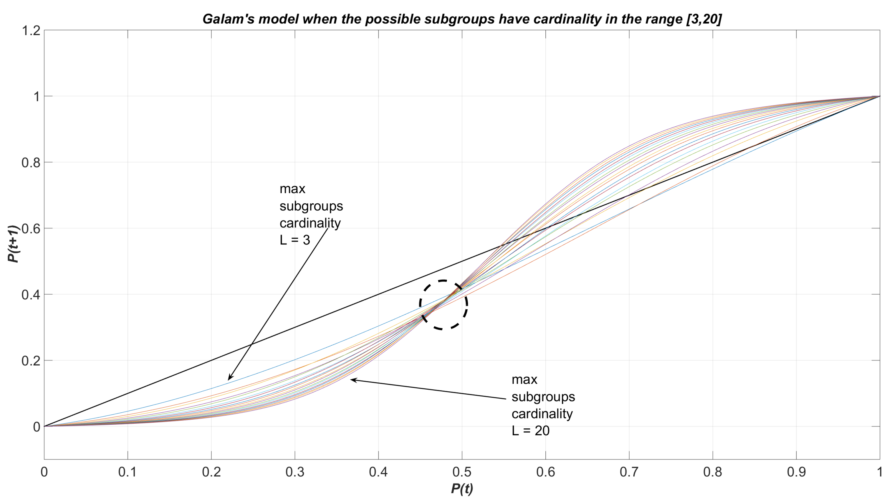
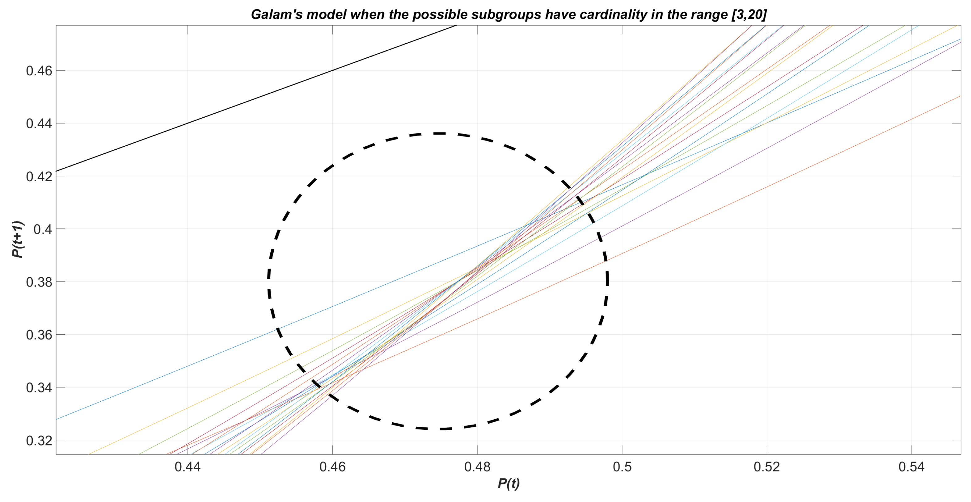
constitutes the threshold value such that when is greater than , then all agents will eventually have opinion ‘+’. Conversely, when all the agents will definitely think ‘−’ if . The value is the fixed point of Equation (1) and is called the killing point or tipping point of the model. In Figure 1, one can observe the dynamics described by relation (1), when the largest cardinality L of the subgroups takes integer values in the interval and , for any k: for each of the 18 curves, the killing point is identified by the intersection with the bisector line other than the extreme points and . Observe that for small values of L no killing point appears (or equivalently, it coincides with the extreme point ). Figure 2 shows a zoomed in perspective of Figure 1.
3. Capturing Additional Dynamics Using a Generalised Galam’s Model
According to model (1), a strict majority of members with positive opinion is a necessary and sufficient condition to have opinion ‘+’ for all the subgroup members.
Since the ultimate choice in a group is frequently the product of a discussion, rather than a simple tally of the two opposing viewpoints in the group, a rule that is so rigorous yet so straightforward could not correctly reflect the actual opinion dynamics in practice. As an illustration, think about the propagation of political opinions. The probability that everyone in the group would share the same view (e.g., +) at the close of a conversation may rise smoothly with the number of members who had that opinion prior to the meeting. As a second application, the reader may consider the audience of social networks, where the dynamics of information spreading was widely investigated in the dedicated literature (see, e.g., [11]).
Accordingly, we suggest to generalise Galam’s model (1) taking into account a softer dynamics of opinion change, i.e., without using rigid majority as a necessary and sufficient condition to shift the entire group to the same view. In particular, we assume that after the conversations, all agents in a group will have opinion ‘+’ with a probability that is dependent on the size k of the group and the number j of agents that had opinion ‘+’ before the discussion. We use the following definition to model the relationship between the probabilities of having an opinion ‘+’ before (i.e., ) and after (i.e., ) discussion (see [12] for a preliminary version of the model):
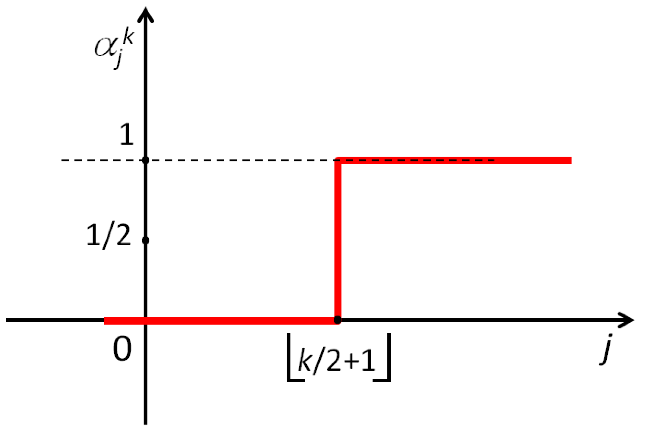
Model (2) generalises model (1), since it is possible to select indeed the probabilities that exactly replicate model (1) (see also Figure 3):
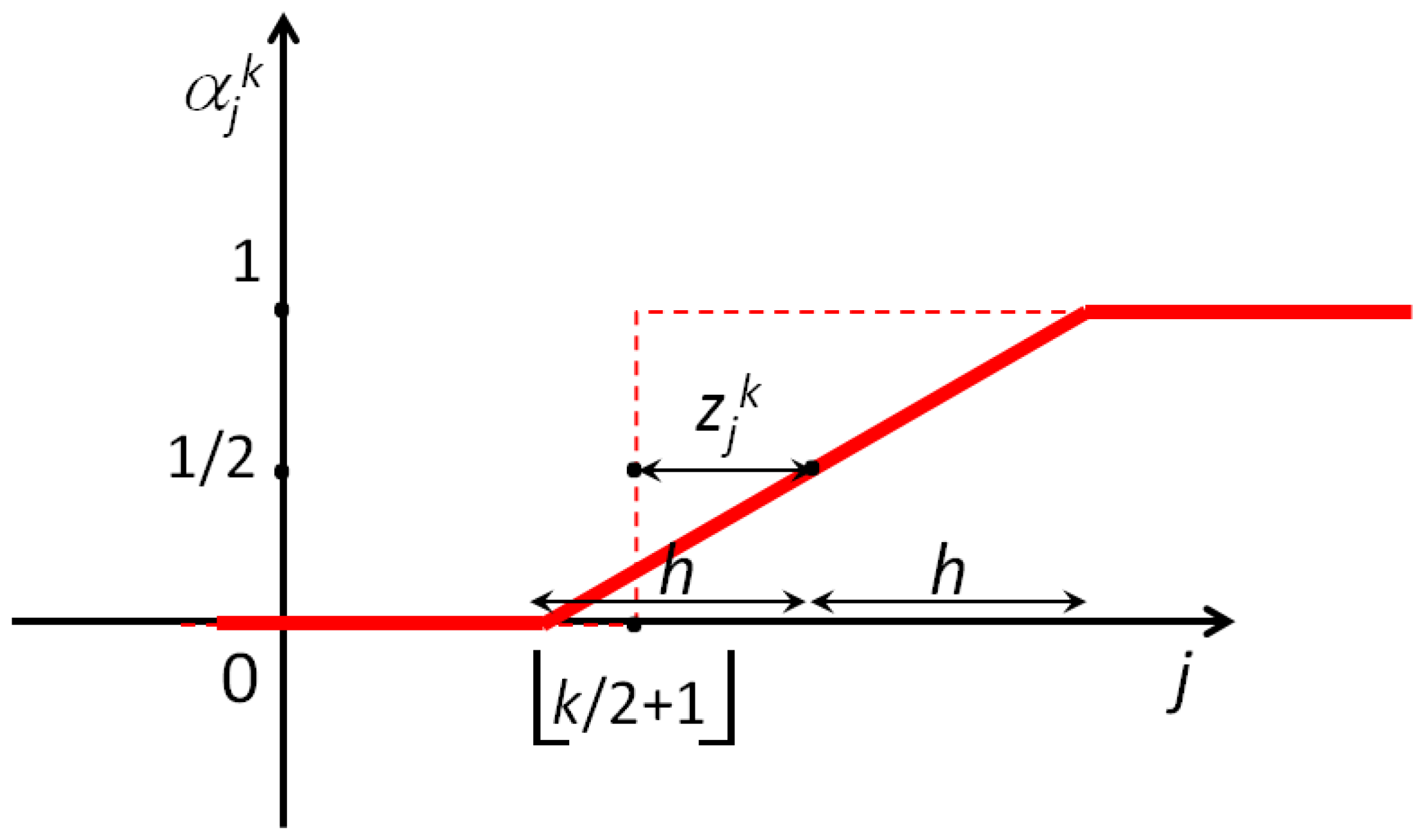
As mentioned, probabilities should reasonably increase with the number j of ‘+’ in a subgroup, and decrease with respect to the size of the group k. In this regard, it is reasonable to expect for the probability to become negligible when the number j of ‘+’ in a subgroup is relatively small (i.e., much lower than the strict majority), and to become close to 1 as the number of ‘+’ noticeably increases (i.e., higher than strict majority). In general, the probability that all agents in the subgroup will adopt the opinion ‘+’ is conceivably a function rising from zero to one as j increases. If one assumes that this function of j is linear, one may precisely define the probabilities as (see Figure 4)
When , the probabilities defined in Equation (4) are exactly the same as in Equation (3). The value of in (4) represents a shift (either positive or negative) from the value , while the slope of the ramp in Figure 4 is .
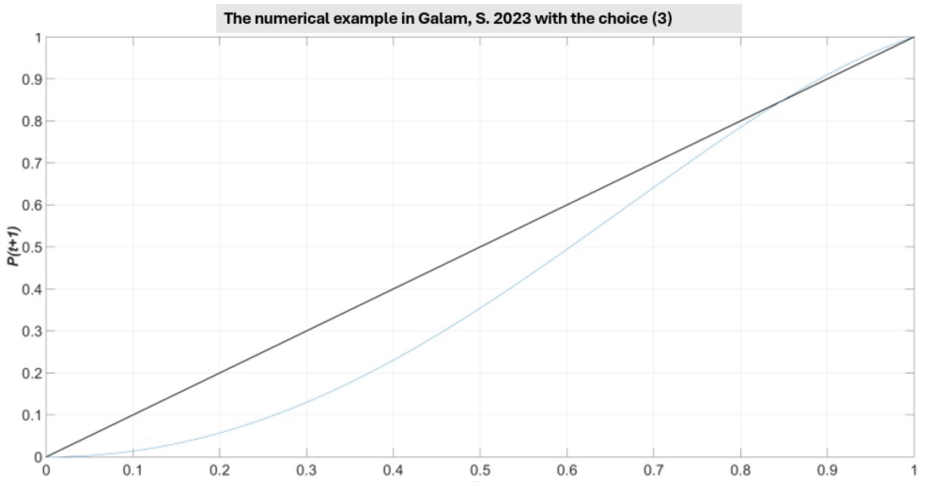
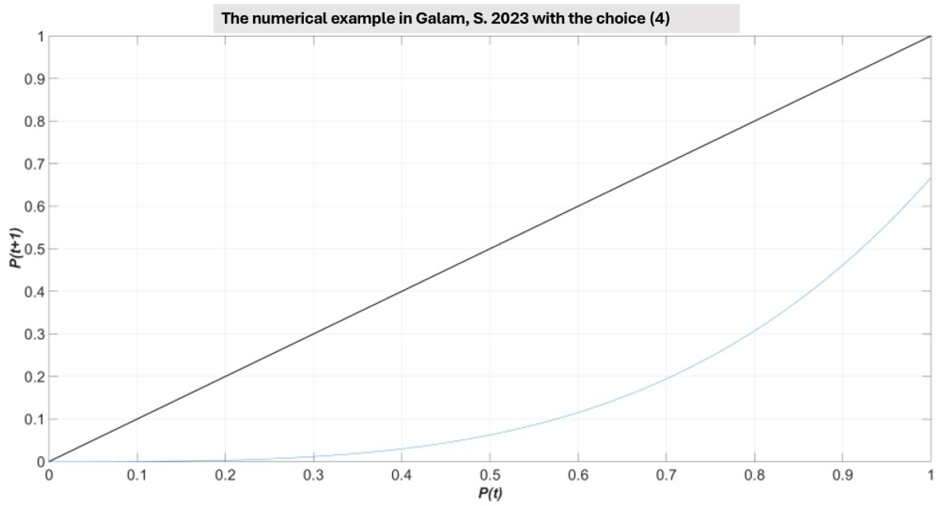
To better grasp the geometric insight behind the choice of the parameters in (4), let us consider the simple numerical example reported in Ref. [6], where , , and (and for all j and k). As reported in Ref. [6], the killing point () lies in between and (see Figure 5). Then, in Figure 6, there is also the model (2) with the choice (4), after setting for any j and k. One can immediately infer that the dynamics of Galam’s model [6] is definitely spoiled when the choice for the coefficients in Equation (3) is replaced by Equation (4). Equivalently, even in case (complete consensus among agents to think +) then the choice (4) imposes a regression towards the stable point given by the origin.
Hence, the presence of a killing point for Galam’s model seems to be strictly related to the expression (1), and introducing the coefficients definitely also spoils the killing point. Moreover, one observes that, in case the majority rule is not explicitly applied in Equation (1), then the dynamics of the model is strongly altered.
Nevertheless, the model (2) retains a number of properties and can suggest fruitful results, following both of the next guidelines:
- it provides clues on the perspective for studying the process of diffusion of information;
- it may suggest proper ways to control information spreading among agents.
At least a couple of intriguing issues in applications can steer the choice of the coefficients , ranging from small–medium- to large-scale (number of agents) applications:
- One Period Analysis. One may assess values for so that, considering at time t the probability , one miximizes the probability at time . In this regard, the values represent costs for steering the information among agents and fostering the positive opinion: the larger (i.e., higher costs) the larger the probability to convey a group to opinion ‘+’. Certainly, the combination of the proper values for each of the coefficients is strongly related to the value , the probabilities , and the binomial coefficients ;
- Multi-Period Analysis. Similarly to the previous item, one may decide to select such that, considering again at time t the probability , one miximizes the probability at time , and compute the entire sequence of intermediate probabilities.
The last two scenarios can be declined in a variety of contexts, including production and marketing, where consumers play the role of agents and the aforementioned perspectives may be the answer to the question: what is (if any) the necessary extra effort in terms of advertising campaign, in order to promote a certain spread of the products or customers’ expectations on items? In this regard, the quantities summarise the resulting effort, while from a mathematical programming perspective they represent unknowns to be assessed. This also suggests that a number of additional questions may arise adopting the model (2), mapping relevant practical instances where a tentative forecast is sought in order to plan the use of (possibly scarce) resources to control the process of diffusion of the information. For the sake of brevity, we itemise below some proposals that are representative but not exhaustive:
- Feasibility Problem. Given the value of and the target value , one may determine a set of values for the coefficients such that, starting at t from , at time , ;
- Focus Group Problem. Given the value of and the target value and the time , one may be interested to determine a set of values for the coefficients such that , where are possible bounds, and . This scenario models a specific interest on those subgroups of cardinality k.
4. Single Period Maximisation of Diffusion
As from the analysis in Section 3, one of the possible proposals to couple the dynamics described through the model (2) with a single period optimisation framework, is given by the following LP scheme:
The last optimisation problem assumes that the value is given, so that both the objective function and the constraints are linear in the set . Though the meaning associated with the objective function is relatively clear, for the constraints some clarifications seem necessary:
- the constraints in Equation (6) state that for a given dimension k of a subset, larger values of the number of agents thinking ‘+’ imply a larger probability ;
- similarly, in the constraints in Equation (7), when the number of agents thinking ‘+’ remains constant, the larger the set cardinality (i.e., k), the smaller the probability ;
- the constraint in Equation (8) expresses the overall cost (i.e., it is a budget constraint) allowed to assess the probabilities , at time t;
- since the quantities need to represent probabilities, they are required to fulfill also the constraint (9).
In order to avoid either infeasible or straightforward solutions for the optimisation Problems (5)–(9), the following lemmas gives some indications on the choice of the parameter , for any t (for a proof, see [12]).
Lemma 1.
Note that Lemma 1 gives a straightforward idea of the fact that the solution of the linear Programs (5)–(9) is substantially nothing else but a generalisation of Equation (1). Furthermore, the next result will give a precise indication on the possible values for the budget in Equation (8).
Lemma 2.
Note that the right sides of Equation (11) explicitly give some hints for the selection of the parameter in Equation (8), both whether in case L it is even or it is odd.
Regarding some technicalities associated with the solution of the optimisation problems (5)–(9), one observes that it is a continuously differentiable problem, where all the functions are linear. Hence, it is a convex problem, so that the set of all its solutions (possibly an empty set or a singleton) is a convex set. This implies that for any given pair of its solutions, all the points in the segment joining them will be solutions, too. Moreover, being a linear program, all its (possible) solutions will lie on vertices of the feasible set, and not in the interior of the feasible set. As is known, this makes its solution relatively simple (throughout any solver based on the simplex method) and achievable in polynomial time. Hence, large-scale instances are well tractable and allow for a scalable solution in a number of applications with a great number of agents (e.g., problems involving social media or large social groups).
We complete this section highlighting that one further generalisation of the linear programs (5)–(9) suggests to disaggregate the budget constraint and to replace the inequality (8) by the set of constraints,
Observe that the value , for any k, represents a budget devoted to possibly affect the solution after working uniquely on the subsets of cardinality k. This increases the flexibility of the model without compromising its overall complexity (being the resulting model yet a linear program).
5. Preliminary Numerical Experience
This Section is devoted to provide a numerical experience where the potentialities of the formulations (5)–(9) are exploited. In this regard, the investigation here is limited to a couple of meaningful instances. The first one is a small-scale (number of unknowns) problem, while the second one attempts to scale the first’s by 100.
5.1. Small-Scale Instance
Regarding the value of the coefficients in (5)–(9), we consider for the small-scale instance the following setting:
The above choice corresponds to possibly allow only subgroups of dimensions 1, 3, 5, 7, and 9, with probabilities that include null values and possibly repeated values. Furthermore, we set the initial percentage of the population thinking ‘+’ to . Finally, in order to avoid an empty feasible set in Equations (5)–(9) we also selected, respectively, the values and , based on Lemma 2. The outcomes of our numerical experience are obtained using the solver CPLEX 20.1.0.0 available on the NEOS Server platform [13]. Let us remark that CPLEX is definitely among the best and faster solvers for LP, along with the alternative solver BARON. Our numerical experience on the above two instances is summarised as follows:
- : the problems (5)–(9) is coded using AMPL (A Mathematical Programming Language; see [14,15]). The presolve tool in CPLEX eliminated 65 constraints from the formulation, so that the simplified problem was reduced to 65 variables and 110 linear inequality constraints. Regarding the final solution, CPLEX performed 13 dual simplex iterations (i.e., iterations of a method for LP which represents the counterpart of the simplex method, after exploiting the duality theory), with an overall time for the solution not larger than a couple of seconds. Finally, the value of found by the solver iswith the set of variables given by
k = 1 k = 2 k = 3 k = 4 k = 5 k = 6 k = 7 k = 8 k = 9 k = 10 j = 0 0 0 0 0 0 0 0 0 0 0 j = 1 1 0 0 0 0 0 0 0 0 0 j = 2 . 0 0 0 0 0 0 0 0 0 j = 3 . . 2/3 2/3 2/3 0 0 0 0 0 j = 4 . . . 2/3 2/3 0 0 0 0 0 j = 5 . . . . 2/3 0 0 0 0 0 j = 6 . . . . . 0 0 0 0 0 j = 7 . . . . . . 0 0 0 0 j = 8 . . . . . . . 0 0 0 j = 9 . . . . . . . . 0 0 j = 10 . . . . . . . . . 0 - : again the problem (5)–(9) is coded using AMPL and the presolve tool in CPLEX eliminated 65 constraints from the formulation, so that again the simplified problem was reduced to 65 variables and 110 linear inequality constraints. CPLEX performed 18 dual simplex iterations with an overall time for computation similar to the case where it is . Finally, the value of found by the solver iswith the set of variables given by the matrix,
k = 1 k = 2 k = 3 k = 4 k = 5 k = 6 k = 7 k = 8 k = 9 k = 10 j = 0 1 0 0 0 0 0 0 0 0 0 j = 1 1 0 0 0 0 0 0 0 0 0 j = 2 . 0 0 0 0 0 0 0 0 0 j = 3 . . 1 1 1 0 0 0 0 0 j = 4 . . . 1 1 0.285714 0.285714 0 0 0 j = 5 . . . . 1 0.285714 0.285714 0 0 0 j = 6 . . . . . 0.285714 0.285714 0 0 0 j = 7 . . . . . . 0.285714 0 0 0 j = 8 . . . . . . . 0 0 0 j = 9 . . . . . . . . 0 0 j = 10 . . . . . . . . . 0 Note that while allowing a larger value of the budget (for example, ), the solver is able to select a larger number of nonzero unknowns, so that the final value of is almost doubled with respect to the case . In actual applications, this implies that, in order to obtain almost twice the effect of the previous case, on this instance twice the value of the budget must be allowed.
5.2. Large-Scale Instance
Here, we focus on the same instance of Section 5.1, where conversely, a larger number of unknowns is considered. The novel setting of the parameters for the solver are given as follows:
The above choice corresponds to possibly allow all the subgroups with the same probability, and again the initial percentage of the population thinking ‘+’ is equal to . Similarly to the small-scale instance, we consider two values for the budget, and . The computation is again performed adopting the solver CPLEX 20.1.0.0 on the NEOS Server [13]. The outcomes of the resulting two instances are summarised as follows:
- : the problems (5)–(9) is coded using AMPL and the presolve tool in CPLEX eliminated 501,500 constraints from the formulation. The overall simplified problem contained 501,500 variables and 1,001,000 linear inequality constraints. CPLEX performed 192 dual simplex iterations with a time of computation smaller than 20 s, showing that the linear model can well scale the time of computation. The final value of found by the solver iswith the set of variables given by
k = 1 k = 2 k = 3 k = 4 k = 5 k = 6 k = 7 k = 8 k = 9 k = 10 k = 11 k = 12 k ≥ 13 j = 0 1 0 0 0 0 0 0 0 0 0 0 0 0 j = 1 1 1 1 0 0 0 0 0 0 0 0 0 0 j = 2 . 1 1 1 1 0 0 0 0 0 0 0 0 j = 3 . . 1 1 1 1 1 0 0 0 0 0 0 j = 4 . . . 1 1 1 1 1 0 0 0 0 0 j = 5 . . . . 1 1 1 1 1 1 0 0 0 j = 6 . . . . . 1 1 1 1 1 1 0 0 j = 7 . . . . . . 1 1 1 1 1 0.8333 0 j = 8 . . . . . . . 1 1 1 1 0.8333 0 j = 9 . . . . . . . . 1 1 1 0.8333 0 j = 10 . . . . . . . . . 1 1 0.8333 0 j = 11 . . . . . . . . . . 1 0.8333 0 j = 12 . . . . . . . . . . . 0.8333 0 j = 13 . . . . . . . . . . . . 0 j = 14 . . . . . . . . . . . . 0 j > 14 . . . . . . . . . . . . 0 - : the outcomes are quite similar to the case where , with 501,500 indicating the overall number of variables and 1,001,000 the linear inequality constraints. CPLEX performed 30,854 simplex iterations with a time of computation smaller than 20 s, showing again that the linear model can well scale the time of computation. The final value of found by the solver was nowand we do not report the value of the unknowns for the sake of simplicity.
Observe that in both the last two examples, given that subgroups are allowed to be quite large, despite relatively high budget values, the levels reached by the probabilities are quite low.
As a general achievement, we can immediately describe the pattern of the nonzero unknowns which was respected in all four numerical tests reported above. In particular, we can prove that the solution of the formulations (5)–(9) only fills the principal submatrix of unknowns of order , depending h on the value of the budget parameter along with the number of possible subgroups L. Finally, this also allows one to straightforwardly assess a number of null unknowns and possibly reduce the complexity of the overall formulation.
6. A Multi-Period Model
This Section considers a multi-period reformulation of the LP (5)–(9), in order to further generalise the model (2). In particular, in place of the single-period model (5)–(9), where at time step t the quantity is maximised starting from , we can consider a multi-period approach with the ultimate goal of maximising , where T is the time horizon. The latter approach is summarised in the following Nonlinear Program (NLP):
The above NLP includes the unknowns
which represent a larger number of variables with respect to Equations (5)–(9). This implies that the larger the time horizon T, the larger the number of unknowns of the resulting problem formulation. Moreover, as already remarked, Equations (12)–(17) represents an NLP, which in general increases the difficulty of its solution. In particular, the nonlinearities in Equation (13) might yield a nonconcave overall maximisation problem, which implies that a certain number of local maxima (which are not global) might arise. In addition, unlike Equations (5)–(9), the feasible set of Equations (12)–(17) is no longer a polyhedron, so that the final solutions are not necessarily located on the boundary of the feasible set. As a consequence, the choice of the starting value in Equation (13) becomes a key factor for at least a couple of reasons:
Regarding the constraints in Equation (13), observe that the constraints just state a recursion for the function in Equation (2), at each time step. Moreover, the constraints in Equations (14), (15), and (17) have a similar meaning of the constraints in Equations (6), (7), and (9), for the single-period formulation. Finally, the budget constraints in Equation (16) have a possible double formulation, due to the multi-period scheme.
Proposition 1.
Proof.
Observe that from relation (2), one has the following equalities:
Thus, considering that is a constant value, the maximisation in Equation (12) is equivalent to the maximisation,
Moreover, observe that if is given, depends only on the unknowns,
and the maximisation in Equation (5) is equivalent to
Now, suppose the sequence is a solution of Equations (5)–(9); then, it also satisfies Equation (13) for t, as well as Equation (14)–(17). Thus, if the sequences,
solve the problem (5)–(9), for , then by Equation (18), the values in Equation (19) are a feasible point of Equations (12)–(17), satisfying also Equation (18), i.e., Equation (19) is a solution of Equations (12)–(17). □
Lemma 3.
Proof.
The proof trivially follows the guidelines of the proof for Proposition 1. □
Lemma 4.
Proof.
The convexity of and the hypotheses imply
so that also satisfy Equation (21). The rest of the proof follows the guidelines of the proof for Proposition 1. □
Remark 1.
A Numerical Example
We provide here a preliminary numerical example, where the solution of the formulation (12)–(17) is considered, and the budget constraints (16) are replaced by the unique one (which aggregates possible different budgets at the epoches ):
Since the multi-period formulation is indeed nonlinear and possibly nonconvex, we preferred to preliminarily investigate its solutions through a renowned nonlinear (NLP) solver from the literature. In particular, we adopted Knitro 13.2.0 from the NEOS Server [13]. Nevertheless, we are aware that since the problem might be nonconvex (unless the last property is explicitly proved to hold for Equations (12)–(17)), the choice of the starting point by the NLP solver may be crucial, to both outreach an accurate final solution and to reduce the overall computational burden. The parameters of the two instances considered are summarised as follows (respectively):
and
In what follows, we briefly show that, due to the smaller budget (i.e., ) in the first scenario, it yields worse results (i.e., a smaller value of ) with respect to the second scenario. Indeed, adopting the first set of parameters for our multi-period formulation, Knitro presolver was able to eliminate 403 constraints and 1 variable, so that the final formulation included 395 variables and 660 constraints. Moreover, for the probabilities , we obtain the following nonmonotone sequence (due to the nonlinearity of the multi-period model)
Conversely, adopting the second set of parameters for our multi-period formulation, Knitro presolver was again able to eliminate 403 constraints and 1 variable, yielding for the probabilities the values
Again, one observes a nonmonotone behaviour for the sequence , due to nonlinearities of the multi-period model. For the sake of completeness let us remark that the solution of the last two nonlinear instances by Knitro required no more than 10 s each.
7. Conclusions
In this paper, we studied the problem of possibly enhancing standard dynamics from sociophysics (namely the model (1)), using a mathematical programming perspective. We were interested about following a couple of lines of research. First, we coupled the model (1) with an LP scheme in order to possibly control the probability for a given probability , after leveraging the unknowns in Equation (2). The final value of these variables gives a measure of the effort which is required to steer the diffusion process of the opinion ‘+’ for the subgroups of cardinality k. The dynamics are strongly based on the idea of possibly maximising . A numerical experience is also reported in this regard, showing that the computational effort for solving LPs associated with this first proposal is definitely modest, even in the case where the solution of large instances is sought.
As a second task, we also extended the (one period) LP formulations to a more general multi-period formulation, and in this case it was necessary to compute the sequence for a given value of and for a given time horizon, T. Some theoretical properties showing a connection between the solutions of both our proposals have been given, though much work yet is required, including a broad numerical experience also in the multi-period case.
Author Contributions
Conceptualization, A.E., G.F. and D.F.; Methodology, A.E., G.F. and D.F.; Software, A.E., G.F. and D.F.; Validation, A.E., G.F. and D.F.; Writing—original draft, A.E., G.F. and D.F.; Writing—review & editing, A.E., G.F. and D.F. All authors have read and agreed to the published version of the manuscript.
Funding
G.F. wishes to thank the CNR-INM—Institute of Marine Engineering, Italian National Research Council, and the GNCS (Gruppo Nazionale per il Calcolo Scientifico) group within INdAM (Istituto Nazionale di Alta Matematica “Francesco Severi”), Italy, for their support.
Data Availability Statement
Not applicable.
Conflicts of Interest
The authors declare no conflict of interest. The funders had no role in the design of the study; in the collection, analyses, or interpretation of data; in the writing of the manuscript; or in the decision to publish the results.
References
- Bass, F.M. A new product growth for model consumer durables. Manag. Sci. 1969, 15, 215–227. [Google Scholar] [CrossRef]
- Moore, G.A. Crossing the Chasm: Marketing and Selling Disruptive Products to Mainstream Customers; Harper Business: New York, NY, USA, 2014; Available online: https://archive.org/details/crossingthechasm_202002/mode/2up (accessed on 5 August 2023).
- Rogers, E.M. Diffusion of Innovations; The Free Press: New York, NY, USA, 2003. [Google Scholar]
- Schelling, T.C. Dynamic models of segregation. J. Math. Sociol. 1971, 1, 143–186. [Google Scholar] [CrossRef]
- Galam, S. Sociophysics: A review of Galam models. Int. J. Mod. Phys. C 2008, 19, 409–440. [Google Scholar] [CrossRef]
- Galam, S. Modelling rumors: The no plane pentagon french hoax case. Phys. A 2003, 320, 571–580. [Google Scholar] [CrossRef]
- Ellero, A.; Fasano, G.; Sorato, A. A modified Galam’s model for word-of-mouth information exchange. Physica A 2009, 388, 3901–3910. [Google Scholar] [CrossRef]
- Ellero, A.; Fasano, G.; Sorato, A. Stochastic model for agents interaction with opinion–leaders. Phys. Rev. E 2013, 87, 042806. [Google Scholar] [CrossRef] [PubMed]
- Galam, S. Sociophysics. A Physicist’s Modeling of Psycho-Political Phenomena; Springer Science + Business Media, LLC: New York, NY, USA, 2012. [Google Scholar] [CrossRef]
- Galam, S.; Jacobs, F. The role of inflexible minorities in the breaking of democratic opinion dynamics. Physica A 2003, 381, 366–376. [Google Scholar] [CrossRef]
- Backstrom, L.; Huttenlocher, D.; Kleinberg, J.; Lan, X. Group formation in large social networks: Membership, growth, and evolution. In Proceedings of the 12th ACM SIGKDD International Conference on Knowledge Discovery and Data Mining, Philadelphia, PA, USA, 20–23 August 2006; pp. 44–54. [Google Scholar] [CrossRef]
- Ellero, A.; Fasano, G.; Favaretto, D. An application of Linear Programming to sociophysics models. In Proceedings of the Modeling and Analysis of Complex Systems and Processes, Venice, Italy, 22–24 October 2020; pp. 23–33. Available online: https://ceur-ws.org/Vol-2795/ (accessed on 5 August 2023).
- NEOS Server: State-of-the-Art Solvers for Numerical Optimization. Available online: https://neos-server.org/neos (accessed on 5 August 2023).
- Fourer, R. Modeling languages versus matrix generators for linear programming. ACM Trans. Math. Softw. 1983, 9, 143–183. [Google Scholar] [CrossRef]
- Fourer, R.; Gay, D.M.; Kernighan, B.W. AMPL: A Modeling Language for Mathematical Programming; Duxbury Press/Thomson Co.: Belmont, CA, USA, 2002; Available online: https://vanderbei.princeton.edu/307/textbook/AMPLbook.pdf (accessed on 5 August 2023).
Figure 1.
Dynamic curves described by relation (1), when the largest cardinality L of the subgroups takes integer values in the interval and , for any k.
Figure 1.
Dynamic curves described by relation (1), when the largest cardinality L of the subgroups takes integer values in the interval and , for any k.

Figure 2.
Dynamic curves described by relation (1), when the largest cardinality L of the subgroups takes integer values in the interval and , for any k: magnification of the area of intersections among curves.
Figure 2.
Dynamic curves described by relation (1), when the largest cardinality L of the subgroups takes integer values in the interval and , for any k: magnification of the area of intersections among curves.

Figure 3.
For a given , the model (3) considers the above step-shaped choice for the coefficients . In particular, if then , otherwise , so that this choice corresponds exactly to obtain the original Galam’s model (1).

Figure 4.
For a given , the model (4) considers the above piecewise-linear choice for the coefficients , where represents a shift with respect to the abscissa , and is the slope of the ramp.
Figure 4.
For a given , the model (4) considers the above piecewise-linear choice for the coefficients , where represents a shift with respect to the abscissa , and is the slope of the ramp.


Disclaimer/Publisher’s Note: The statements, opinions and data contained in all publications are solely those of the individual author(s) and contributor(s) and not of MDPI and/or the editor(s). MDPI and/or the editor(s) disclaim responsibility for any injury to people or property resulting from any ideas, methods, instructions or products referred to in the content. |
© 2023 by the authors. Licensee MDPI, Basel, Switzerland. This article is an open access article distributed under the terms and conditions of the Creative Commons Attribution (CC BY) license (https://creativecommons.org/licenses/by/4.0/).
Share and Cite
MDPI and ACS Style
Ellero, A.; Fasano, G.; Favaretto, D. Mathematical Programming for the Dynamics of Opinion Diffusion. Physics 2023, 5, 936-951. https://doi.org/10.3390/physics5030061
AMA Style
Ellero A, Fasano G, Favaretto D. Mathematical Programming for the Dynamics of Opinion Diffusion. Physics. 2023; 5(3):936-951. https://doi.org/10.3390/physics5030061
Chicago/Turabian StyleEllero, Andrea, Giovanni Fasano, and Daniela Favaretto. 2023. "Mathematical Programming for the Dynamics of Opinion Diffusion" Physics 5, no. 3: 936-951. https://doi.org/10.3390/physics5030061