Spatial and Temporal Changes of Tidal Inlet Using Object-Based Image Analysis of Multibeam Echosounder Measurements: A Case from the Lagoon of Venice, Italy

Abstract

Scientific exploration of seabed substrata has significantly progressed in the last few years. Hydroacoustic methods of seafloor investigation, including multibeam echosounder measurements, allow us to map large areas of the seabed with unprecedented precision. Through time-series of hydroacoustic measurements, it was possible to determine areas with distinct characteristics in the inlets of the Lagoon of Venice, Italy. Their temporal variability was investigated. Monitoring the changes was particularly relevant, considering the presence at the channel inlets of mobile barriers of the Experimental Electromechanical Module (MoSE) project installed to protect the historical city of Venice from flooding. The detection of temporal and spatial changes was performed by comparing seafloor maps created using object-based image analysis and supervised classifiers. The analysis included extraction of 25 multibeam echosounder bathymetry and backscatter features. Their importance was estimated using an objective approach with two feature selection methods. Moreover, the study investigated how the accuracy of classification could be affected by the scale of object-based segmentation. The application of the classification method at the proper scale allowed us to observe habitat changes in the tidal inlet of the Venice Lagoon, showing that the sediment substrates located in the Chioggia inlet were subjected to very dynamic changes. In general, during the study period, the area was enriched in mixed and muddy sediments and was depleted in sandy deposits. This study presents a unique methodological approach to predictive seabed sediment composition mapping and change detection in a very shallow marine environment. A consistent, repeatable, logical site-specific workflow was designed, whose main assumptions could be applied to other seabed mapping case studies in both shallow and deep marine environments, all over the world.

1. Introduction

Precise maps of the seabed are critical for the observation and exploration of marine environments, giving the possibility to describe the physical, biological, and geological aspects of the ocean. They are crucial for sustainable management of coastal areas, and for marine spatial planning and benthic habitat mapping, forming a basis for designating the Marine Protected Areas (MPAs) [1]. According to McGonigle et al. [2], there is an immediate need to characterize the type, size, and extent of benthic habitats. The condition of the seabed is indicative of marine environmental quality, which should be monitored and protected due to global warming and mean sea level rise. The development of standardized mapping methods is required to establish good environmental status (GES) of Descriptor D6, Seafloor Integrity, of the European Union Marine Strategy Framework Directive (MSFD; D6 Commission Decision (EU) 2017/848 of 17 May 2017). Maps of the seafloor representing physical, biological, and geological properties are required for preservation of the marine environment and its biological resources. Moreover, the authorities of some countries are aware of seafloor exploration, establishing national mapping programs, such as RITMARE, MAREANO, MAREMAP, AusSeabed, and INFOMAR [3,4,5].

Benthic habitat mapping could be defined as follows—“plotting the distribution and extent of habitats to create a map with complete coverage of the seabed showing distinct boundaries separating adjacent habitats” [6], keeping in mind the possible limits in the definition of these boundaries [7,8]. This multidisciplinary approach links knowledge from oceanography, underwater acoustics, ecology, sedimentology, geomorphology, statistics, geoinformation, and numerical modeling. Benthic habitat mapping often means analyzing and interpreting hydroacoustic and ground truth datasets, including developing integration methods between continuous coverage geospatial datasets and in situ point measurements [6,9].

Despite the recent rapid development of hydroacoustic devices and tools for geomorphometric analysis, detection of spatial and temporal changes of benthic habitats over time was only recently investigated [10,11,12,13,14,15]. The main measuring device used for high-resolution spatial mapping of the seafloor is the multibeam echosounder (MBES) [16]. It allows us to measure bathymetry and backscatter responses of the seabed that reflect the seafloor substratum types. Whereas acquisition of MBES bathymetry is standardized for hydrographic purposes, backscatter of acoustic signal from the seabed is much more complicated, due to factors like variations of the seabed substratum, environmental properties, different sonar characteristics, and applied acquisition settings. In order to track spatial and temporal changes of seafloor sediments, the recent development of MBES devices is heading towards calibration of MBES backscatter. Therefore, the majority of MBES change detection studies concentrate on the temporal reliability of MBES backscatter levels [5,14]. This allows us to perform relative calibration on the natural reference areas of known and stable acoustic properties. Other methods assume absolute calibration of MBES backscatter, by cross-calibration with calibrated devices, like a single-beam echosounder [17]. In this research, we conducted two separate surveys, using MBES uncalibrated in terms of acoustic backscatter. For each survey, we collected separate ground-truth datasets that were used for automatic supervised classification.

As underwater acoustic datasets become larger and more detailed, there is a need for efficient methods of automatic classification of heterogeneous benthic habitats, to reduce the time of data analysis and ensure repeatability [6]. Despite the progress made in recent years, acoustic seafloor classification and monitoring using reproducible, automated methods is still in its infancy. Therefore, benthic habitat mapping is currently strongly focused on methodological developments, and different approaches have been applied to classify backscatter mosaics—pixel-based and object-based analysis [18,19,20] using supervised and unsupervised image classification [21,22,23]. The use of a remote sensing approach like object-based image analysis (OBIA) to improve the accuracy and understanding of seafloor classification recently received much attention [24,25]. However, these automated methods were applied in only a limited way to detect sediment composition changes over time [11]. Therefore, one of the main purposes of this paper was to supplement existing change detection methodology with object-based image analysis of multibeam echosounder measurements.

This work aimed to—(a) develop the best OBIA procedure to analyses multibeam time-series datasets; (b) investigate how classification accuracy could be affected by the scale of object-based segmentation; and (c) assess the accuracy of the classification and its potential to detect changes in seafloor composition. The tested OBIA procedure would not only provide insights on local changes related to the construction of large coastal infrastructure in the Venice Lagoon inlet, but would also be a basis for the development of automated approaches to assessing seafloor change detection, in view of more efficient mapping opportunities (i.e., through autonomous underwater vehicles or other robotic systems) and the increasing importance of seafloor monitoring, all over the world [26,27].

2. Materials and Methods

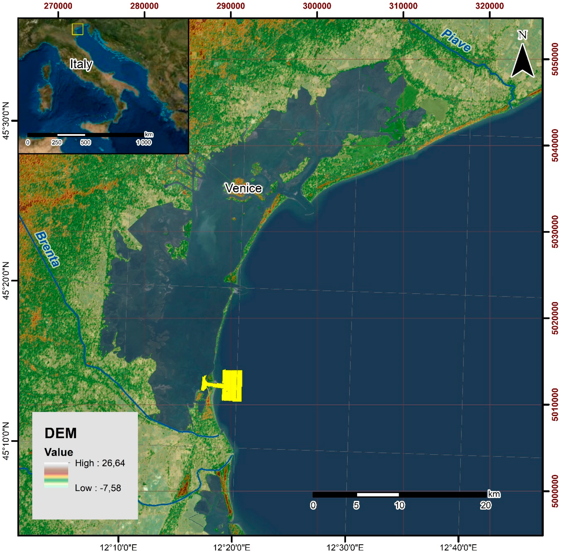
The following three subsections consider the study area and descriptions of MBES and ground-truth data acquisition. Further subsections cover processing details developed in this study.

2.1. Study Area

The Lagoon of Venice is located in the northwest part of the Adriatic Sea (Figure 1). The historic city of Venice together with its surrounding lagoon became a UNESCO World Heritage Site in 1987. Its area of about 550 km² makes it the largest lagoon in the Mediterranean Sea. The mean depth of the lagoon is around 1.2 m, with a maximum depth of 30 m [28]. The lagoon has three inlets (Lido, Malamocco, and Chioggia) that connect it with the open sea (Figure 1). Moreover, the lagoon consists of a complicated network of navigation channels, tidal channels, intertidal mudflats, and intertidal salt marshes [29]. Areas deeper than 5 m make up only 5% of the area, and areas shallower than 2 m make up around 75% [30]. Centuries of high anthropogenic pressure impact the dynamic and fragile ecosystem of the lagoon (e.g., [31]), representing one of the main causes of an increasing sinking rate and catastrophic floods in the last and current centuries [32,33]. To prevent the city from exceptional high tides, the Modulo Sperimentale Elettromeccanico (MoSE; Experimental Electromechanical Module) project was established in 2002. The project led to the development of mobile barriers located at the three inlets connecting the lagoon with the open sea [34,35]. The 79 elements of the mobile barriers are raised whenever marine water exceeds a specified level (for now, 110 cm). Considering predictions of sea level rise in the next few decades, the MoSE system was designed to protect the lagoon from tides of up to 3 m [35]. Such hard anthropogenic structures located in the inlets could substantially affect the hydrodynamics, sediment transport, and the benthic habitat distribution of the lagoon [36]. In particular, it was shown that the recent construction of the hard structures had a direct impact on the seafloor [15,37]. Hence, there is a pressing need to understand the spatial and temporal response of the seafloor.

From the hydrodynamic point of view, the Lagoon of Venice is a micro tidal basin [30]. After crossing the main inlets, the tide enters major channels and reaches shallow flats and salt marshes. Major wind systems that occur over the Adriatic Sea, like bora and sirocco, have a significant impact on the region’s hydrodynamics. Besides exceptional conditions, sea level changes during astronomical tides often vary around 1.0 m for spring tides. The oceanographic conditions of the lagoon lead to salinity ranging between 20 and 35 PSU, with an average of 30.18 PSU, while temperature ranges from 8 to 25 °C, with an average of 17.6 °C [30].

The Chioggia area of interest (AOI) was greatly modified by human activity over the centuries, though it underwent the most significant changes due to the development of the MoSE project, similar to the Lido inlet [15]. The southernmost inlet of the lagoon had an average depth of around 8 to 12 m in artificially maintained navigation channel areas [36]. The width of the inlet was 350 m in the narrowest part and its length was 2 km. Between 2003 and 2006, a curved seaward breakwater was created and the inlet channel width was reduced. The presence of the breakwater separated the outgoing flow into the two branches. The separation caused an increase of current speed, resulting in augmented erosion of the seabed and sediment transport [37]. Inside the inlet, many morphological features like scour holes, dune fields, megaripples, and rip-rap were mapped. On the landward side of the inlet, the presence of larger structures like flood- and ebb-tide deltas was documented [38,39].

2.2. MBES Data Acquisition

Acoustic datasets of the seafloor were collected in 2013 and 2016 by scientific surveys, using a multibeam echosounder under the RITMARE research project (a national research program funded with support by the Italian Ministry of Education, University, and Research). The main survey campaign was conducted for 17 weeks in May–December 2013 [5]. An approximately 10 km² part of the main research area in the Chioggia inlet was covered in November–October 2013. An additional survey covered the inlet in September 2016. All surveys were conducted onboard the R/V LITUS, with a draught of 1.6 m.

Investigation of the Chioggia inlet was done using a Kongsberg EM 2040 DC MBES mounted on a pole at the bow of the ship. The whole measuring system contained the MBES and components including a Kongsberg Seatex Motion Reference Unit 5 (MRU 5), two Global Positioning System (GPS) sensors mounted at the dual antenna, and a sound velocity sensor (SVS; Valeport). Internal devices were mounted inside the ship—the processing and human–machine interface (HMI) unit, a Fugro HP differential GPS (DGPS), and a sound velocity profile (SVP) Smart–X measuring probe (AML Oceanographic). The motion reference unit, DGPS, and processing and HMI unit are core components of the Kongsberg Seapath 300 system. An MRU 5 inertial sensor provided precise measurements of the linear and rotary movements in three dimensions. Two GPS receivers mounted on the antenna provided high-quality measurements of position and velocity. DGPS accuracy reached 0.2 m, the accuracy of pitch and roll was 0.02°, and the accuracy of heading was 0.075°. Sound velocity was measured using a Valeport miniSVS mounted near the MBES transducers, collecting data in real-time during vessel movement. Another device, a Smart–X (AML Oceanographic, 2012), provided SVP through the water column. We used the Kongsberg Seafloor Information System (SIS) to log, display, and check acquired data in real-time, onboard the ship.

The Kongsberg EM 2040 DC MBES allowed the acquisition of data for an operating frequency range from 200 to 400 kHz. It had two transducers (heads) equipped with 1600 receiving beams (800 per head, 400 per swath). The MBES beam width was 1 × 1°, and in a dual-head configuration, it could cover up to 200° for frequencies from 200 to 320 kHz.

The surveys were performed after field calibration of the MBES parameters and regular tests [5]. The reliability of MBES backscatter measurements for this research was estimated in [5]. To ensure an MBES dataset with the best possible quality, transect lines were planned with 40% overlap between the neighboring swaths. The speed of the ship was kept constant at 4 knots. The frequency of transmitted acoustic signals was set to 360 kHz. The number of beams was set to high-density single swath, which meant that there were 800 beams in a dual-head configuration. Swath coverage in the inlets was 105° (60° for each head with 15° overlap). The applied pulse length was 35 μs. Beam widths had dimensions of 1 × 1°. SVP measurements were performed at least every 4 h, more often when there were changing oceanographic conditions, due to, for example, transfer to another water body.

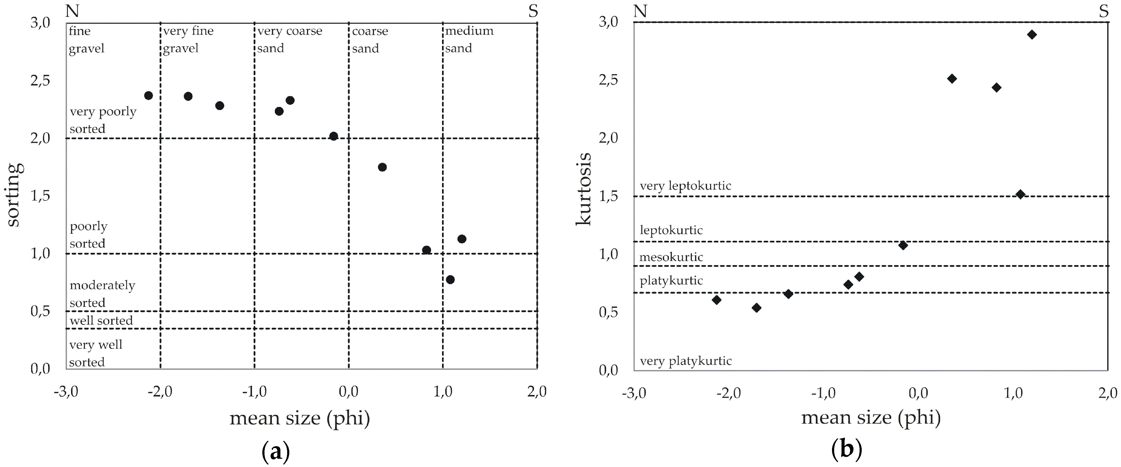
2.3. Ground Truth Samples

Ground truth samples collected in the AOI included superficial sediment samples and seabed photographs. They were acquired, analyzed, and described by CNR–ISMAR for 2012–2016, using methods described in the following paragraphs. Ground truth samples were taken in the chosen sites with representative MBES backscatter and bathymetry characteristics. After being analyzed and processed, they were used to conduct feature selection, supervised classification, and accuracy assessment of the generated benthic habitat map.

Sediment samples were taken using a 7 dm³ Van Veen grab. In March 2012 and April 2014, 27 and 17 sediment samples were collected, respectively. An additional 29 ground-truth samples were collected in 2016. These were examined using sieve analysis and laser diffraction analysis for finer fractions (smaller than 1 mm), using a Mastersizer 3000 laser particle size analyzer. All samples were classified using Wentworth’s [40] and Folk’s [41] methods, also determining the grain size parameters [42,43]. In the gravel fractions, information about the presence of shell detritus was also included [37].

An aluminum drop frame was designed in the CNR–ISMAR and was successfully used for ground truth in deeper parts of the Chioggia AOI. The drop frame was equipped with a GoPro underwater camera (manufactured by GoPro Inc., 3000 Clearview Way, San Mateo, CA 94402, USA) and two scaling laser pointers, to guarantee appropriate measurements of dimensions. The frame was dropped down from the vessel and allowed to take photos from 40 cm above the bottom, giving a seafloor area of approximately 20 × 25 cm per image. In all, 60 drop frames (3 replicates for 20 stations) were collected in 2014 at the same sites, as sediment samples from the 2014 campaign [37]. Images from photo transects and drop frames were carefully analyzed and inspected by the CNR–ISMAR research team.

2.4. Processing of the MBES Dataset

Kongsberg CARIS HIPS and SIPS software (version 7, manufactured by Kongsberg Gruppen ASA, Kirkegårdsveien 45, NO-3616 Kongsberg, Norway) were utilized to process raw bathymetric and backscatter MBES data, and to create georeferenced grids for further analysis (Figure 2). Bathymetric and backscatter data processing included common steps like sound refraction and tidal corrections. A bathymetric digital elevation model (DEM) was cleaned, removing undesired spikes that might have come from the presence of gas bubbles, schools of fish, etc. Backscatter processing of the Lagoon of Venice utilized the Geocoder engine implementation for backscatter mosaic creation in the CARIS software, allowing angle-varying gain (AVG) correction to be performed for MBES angular dependency [44].

Angle-varying gain is an empirical method that was implemented in the Geocoder software (manufactured by Quality Positioning Services BV (QPS), Handelsweg 6-2, 3707 NH Zeist, Netherlands), to perform angular dependence compensation. As backscatter intensity was significantly dependent on the incidence angle of the seabed, the Geocoder engine allowed correction of all MBES swaths by a moving window, removing the backscatter angular response, creating practical backscatter mosaics for interpretation of the seafloor substratum and mapping of habitats [45]. The choice of an AVG window size was always subjective, as it is a compromise between the presence of artefacts and unification across the multibeam swath [46]. For the study of the Lagoon of Venice, a 300-pixel window size was applied [5]. In order to improve the resulting imagery, we applied a despeckle filter. This tool could filter out noise related to pixels with outstanding grey-level values, similar to a median filter.

The summary workflow covering all processing stages for Chioggia 2013 and 2016 datasets, is shown in Figure 2.

2.5. Feature Extraction

Pixel- and object-based secondary features were created, based on processed MBES bathymetry and backscatter. We extracted 25 secondary derivatives, as shown in

Table 1. List of bathymetry and backscatter intensity features extracted in this study. BPI—bathymetric position index; GLCM—grey-level co-occurrence matrix.

ID	Bathymetry Feature	ID	Backscatter Intensity Feature
1	Rugosity	17	Backscatter standard deviation
2	Slope	18	GLCM mean
3	Variance	19	GLCM standard deviation
4	Aspect	20	GLCM entropy
5	Eastness	21	GLCM homogeneity
6	Northness	22	GLCM contrast
7	Curvature	23	GLCM correlation
8	Planar curvature	24	GLCM angular second moment
9	Profile curvature	25	GLCM dissimilarity
10	Small-scale BPI
11	Large-scale BPI
12	Bathymetry standard deviation
13	Rugosity standard deviation
14	Slope standard deviation
15	Small-scale BPI standard deviation
16	Large-scale BPI standard deviation

. Unless otherwise stated, a 3 × 3 kernel size of the focal neighborhood scanning window was used for calculation of all pixel-based derivatives. These were created using the Benthic Terrain Modeler (BTM) 3.0 Toolbox in the ArcGIS 10.4 software (manufactured by Environmental Systems Research Institute (ESRI), 380 New York Street, Redlands, CA 92373, USA) [47]. Object-based features were determined based on single value per image object in the eCognition 9.0 software (manufactured by Trimble Inc., 935 Stewart Drive Sunnyvale, CA 94085, USA). The features were created based on a multiresolution segmentation algorithm, described in detail in the following section, with the following parameters—shape 0.1, compactness 0.5, and scale factor 5.

The basic statistics used in this study included mean, standard deviation, and variance. As shown in Table 1, standard deviation was calculated for bathymetry, backscatter, rugosity, slope, and bathymetric position index (BPI) at two scales. Considering all pixel values forming the focal neighborhood, variance implied the second moment of their distribution. Standard deviation is equal to the square root of variance [47]. The calculation of slope considered the maximum change in elevation in relation to eight neighbors around a center pixel, based on simple trigonometrical rules [48]. Maximum downslope direction, expressed by the azimuth, could be determined as an aspect [48]. Trigonometric functions allow one to transform an aspect into two alternative measures—northness and eastness [49]. Curvature (slope of slope) is a secondary derivative of bathymetry that was extended with features like planar and profile curvature. Whereas planar curvature is defined as curvature in the direction perpendicular to the maximum slope, profile curvature is calculated along the direction of the maximum slope [50]. Rugosity (ruggedness) was calculated using the vector ruggedness measure (VRM) algorithm, measuring the three-dimensional orientation of pixels inside a focal neighborhood, using vector analysis to estimate dispersion between the vectors and the corresponding pixels [51,52]. BPI measures the difference in DEM between a certain location and the neighboring locations, in relation to the overall bathymetric scene [53]. The scale factor was the general attribute that differentiates BPI results, allowing separation of fine and broad features, which helps in specifying geomorphological structures of different sizes.

In the object-based approach, standard deviation was calculated as one value for image object from all pixel values forming such an object. Grey-level co-occurrence matrices (GLCMs) [54] were used to create object-based secondary features, providing the spatial characteristics of the backscatter mosaic. Spatial dependence between the neighboring pixels could be described by different co-occurrence matrixes. Calculations were performed using the eCognition software for all pixels included in the image object, along four main symmetrical directions summed together. Values of GLCM homogeneity were calculated on the basis of proximity of the pixel distribution to the GLCM diagonal. The opposite measure to GLCM homogeneity was the GLCM contrast, related to the contrast in intensity between two neighboring co-occurrence pixels. Comparable to contrast, GLCM dissimilarity could be characterized by linear, rather than exponential growth, additionally increasing with the growth of the local contrast area. GLCM entropy was a fundamental GLCM measure. As a measure of randomness, it had the highest value when all matrix elements were equal [55]. GLCM angular second moment, also known as energy or uniformity, comes from a physical term of a rotational acceleration measure and reaches high values for orderly matrices [55]. The GLCM mean measures the weight of the frequency of pixel value occurrence with a specified surrounding pixel value. The GLCM standard deviation was used to determine dispersion around the mean; whereas it considered combinations of values of a certain pixel and surrounding pixels to not be equivalent to the ordinary standard deviation. GLCM correlation was used to calculate the linear dependency between the surrounding grey-level pixels [55]. It provided identical information to semivariance and was almost identical to Moran’s I autocorrelation [56].

2.6. Feature Selection

In this study, we applied two feature selection methods. The first was a built-in embedded feature-selection algorithm inside the classification and regression tree (CART) classifier [57,58,59]. The second was the Boruta wrapper algorithm [60]. Feature selection tools were used to improve the classification performance, get rid of unimportant features, and provide the possibility for better understanding of dependencies between data types.

The embedded CART feature-selection algorithm was performed as a part of CART classification in eCognition software. It allowed us to find the optimal subset of features in the training process of the CART classifier. As a result, an importance table was created with an array of values showing the relative decision power for all important features. The importance of a certain secondary feature was calculated over all splits of this feature in the decision tree [57].

The Boruta feature-selection algorithm, created on the basis of a random forest classifier, was implemented using the R software (manufactured by the R Foundation for Statistical Computing, Vienna, Austria, Wirtschaftsuniversität Wien, Welthandelsplatz 1, 1020 Vienna, Austria). Its operating principle is to find all relevant variables by comparing the importance of the original features with the possible importance that could be obtained at random, calculated with their permuted copies [61]. To perform the Boruta feature-selection algorithm, we extracted values of all considered features over the locations of training samples. Feature importance was calculated based on the R script, using the “Boruta” and “rgdal” libraries [61,62].

2.7. Object-Based Image Analysis: Image Segmentation and Supervised Classification

Image objects (segments) are the fundamental aspects of the object-based image analysis. They allow analysis of the backscatter grid, considering size, shape, relationships, and the hierarchy of the homogeneous areas of the seabed. Such generalization brings to mind human perception in terms of looking at an image in a similar way and recognizing environmental relationships at many scales, but not at a pixel scale [63]. Image objects were created from backscatter layers, using a multiresolution segmentation algorithm in eCognition. Described in detail by Benz et al. [64], multiresolution segmentation separates rasters into distinct regions, based on primary features, like grey tone and shape [65]. The segmentation procedure merges smaller image objects (from one pixel object size) into bigger ones. The aim was to separate areas with minimum internal pixel variability and maximum difference from adjacent objects. Object size and internal variability were determined by a dimensionless scale parameter that could be further defined by relationships between the color, shape, smoothness, and compactness of the resulting image objects. Color and shape as well as smoothness and compactness were grouped into weighted pairs, so we needed to define only one value for each pair. We determined multiresolution segmentation parameters with shape 0.1 and compactness 0.5, similar to other OBIA benthic habitat mapping studies [18,66,67,68]. As the scale of multiresolution segmentation was the base initial parameter responsible for further image analysis, we tested different scales from 1 to 60.

Supervised classification is strongly related to supervised learning and machine learning. In machine learning nomenclature, it meant generating an inferred function after analyzing the labeled training sample data [69]. Supervised classification could be separated in two general steps. First, the training samples were used to train a classifier algorithm, to learn the dependencies and relationships between the data. In the second step, the trained classifier algorithm used the inferred function to map the unclassified areas in the most correct and reasonable way possible. The performance of the classifier could then be evaluated using validation samples in the subsequent accuracy assessment step. Under the assumption that there is no single machine learning classifier that is always the best in all supervised classification problems [70], we compared five supervised classifiers to produce seabed composition maps—classification and regression trees (CARTs) [57], random forest (RF) [71], Bayes, support vector machine (SVM) [72], and the K-nearest neighbors (KNN) [73].

CART, introduced by Breiman et al. [57], allowed the classification of data based on recursive partitioning into more uniform groups. The method determined the final classification by utilizing decision trees related to a system of questions and answers. RF is a machine-learning method that is an extension of the previous one, through the development of multiple decision trees and random sets of variables. Using many trees (generally called a forest) usually allows high performance. SVM, another machine-learning algorithm, classified the data using so-called hyperplanes in higher-dimensional space. Support vectors were located in the closest neighborhood to the hyperplane and were used as key vectors to separate the dataset with the largest possible margin in higher-dimensional space. KNN considered a defined number (k) of known training samples to classify the object based on the Euclidean distance from the query point. Bayes, one of the simplest classifiers, produced simple decision rules, assuming normal and independent distribution of all features. The algorithm calculated mean vectors and covariance matrices for each class and required only small amount of training data [23].

2.8. Evaluation of Performance

We used the validation subset of ground truth samples to evaluate the classification results. Accuracy assessment measures were determined based on an error matrix showing cross-tabulation among classified maps and validation samples belonging to each class [74]. The common measures of accuracy assessment used in this study were user’s, producer’s, overall, and kappa. User’s accuracy was a ratio between correctly classified instances to sum up all ground truth possibilities, and producer’s accuracy was the probability of correctly classified reference pixels, compared to all classified pixels. Overall accuracy was the sum of the major diagonal of an error matrix, divided by the total number of instances in a confusion matrix [75,76]. Kappa was a measure that considered all elements of the error matrix [77]. Whereas the range of the kappa coefficient was equal to [−∞,1], it could, in practice, be interpreted as: <0.2 = poor, <0.4 = fair, <0.6 = moderate, <0.8 = good, and close to 1 = very good [8,78].

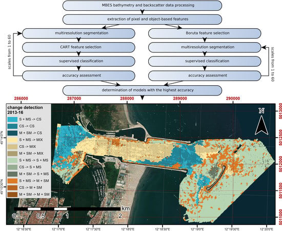
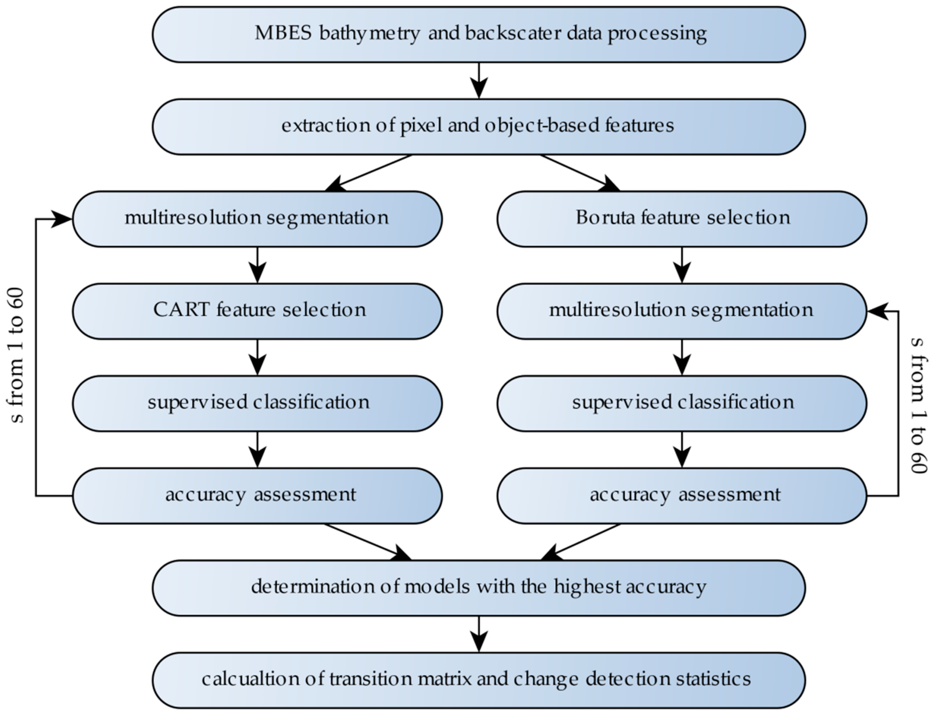
2.9. Change Detection

Change detection is a typical term used in the quantitative analysis of multitemporal spatial data. It tries to explain changes caused by environmental processes, allowing for the observation of spatial changes of habitats at different time steps. In this study, we assessed seafloor sediment changes, based on a transition matrix that included a time-series comparison of “from–to” transitions of every sediment type [79]. While the diagonal of the matrix referred to the persistence of each class, the sum of each class type was related to the total value of time steps. According to Pontius et al. [79], few change detection statistics were extracted from the transition matrix. Gain and loss were related to growth and decrease in area, respectively. Swap referred to a change in spatial location, and net change was defined by the change of quantity of a certain sediment type between time steps [10,11]. Total change was related to the sum of gain and loss for sediment. Quantity change, expressed by the net statistic, was calculated by subtracting the total amount of previous habitat type from the total amount of later sediment category. Additionally, three ratios were provided—gain/persistence (G/p), loss/persistence (L/p), and net/persistence (N/p). These provided information about the tendency of one habitat type to transition to another type. Values of G/p and L/p higher than 1 indicated that the particular class was more prone to gain or loss than other classes. Values close to 0 referred to a lack of change and a strong tendency to persist. The sign of the N/p ratio indicated an overall negative or positive tendency between temporal trends [10,11]. Change detection in this study was performed in ArcGIS, based on the intersection of all sediment areas.

3. Results

3.1. Processing of MBES Datasets

Processing the multibeam echosounder datasets in two time steps, allowed us to generate the bathymetry and backscatter intensity spatial grids presented in Figure 3. Bathymetric layers show geomorphological structures like scour holes and megaripples. Whereas in the western part of the inlet, anthropogenic deepening created a basement for the mobile barriers of the MoSE project, the mouth of the inlet was covered by dune fields. The spatial coverage of the Chioggia 2016 grid was smaller compared to that of 2013; it lacked part of the seaward area, but the inlet itself was fully covered.

A bathymetric comparison between the surveys suggested a similar arrangement of geomorphological structures (e.g., dune field and large dunes at the end of the seaward tidal channel and its foreground) and progressive deepening and extension of scour holes (at breakwater tips).

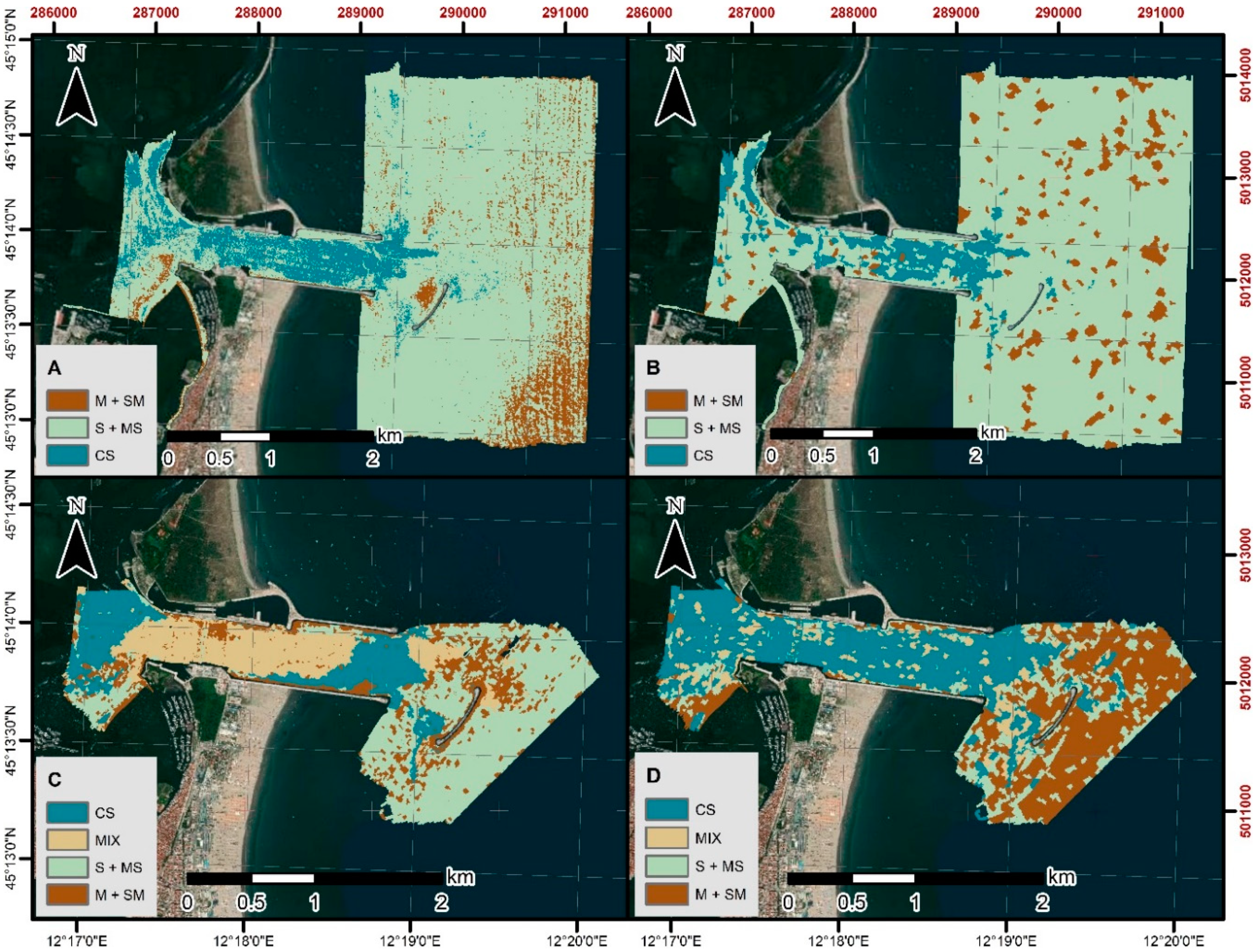
3.2. Identification of Benthic Habitat Classes

We combined the bathymetry and backscatter information with sediment and underwater photo ground truth datasets. This allowed us to determine several classes of sediment, covering specific ranges of backscatter intensity values (

Table 2. Description of the acoustic backscatter of Chioggia 2013 and 2016 areas of interest (AOIs), with corresponding sediment classes and ground truth photographs. CS—coarse sediment; M + SM—mud and sandy mud; S + MS—sand and muddy sand; and MIX—mixed sediment.

MBES Backscatter Image		Class ID	Texture Description	Seabed Image		Seabed Composition
2013	2016			2013	2016
		M + SM	Very low backscatter intensity, gradually changed to other textures			Mud and sandy mud, often covered by benthic vegetation, like Nassarius nitidus, Carcinus astuarii, Spatangidea sp., Veneridae sp.
		CS	High and very high backscatter intensity			Coarse sediment covered by dense benthic detritus and communities of Chamalea, Venerupis aurea, Ostereidae sp., Serpulidae sp., Pectinidae sp.
		S + MS	Low backscatter intensity covering large patches			Medium-grained and muddy sand, rare presence of benthic organisms
-		MIX	Speckled pattern of low and high backscatter intensity	-		Coarse sediment with sand and mud, rarely covered by benthic detritus

). We adopted the simplified European Nature Information System (EUNIS) marine habitat classification scheme, based on a modified folk classification, described by Long [80]. Sediment classes included mud, with the addition of sandy mud (M + SM), coarse sediment (CS), medium-grained sand with the addition of muddy sand (S + MS), and coarse sediment with sand and mud (MIX).

The sedimentological classification of sediments perfectly corresponded to the hydrodynamic regime of the area, which was proposed by [37]. Sediments appropriate for the identified benthic habitats were classified as follows:

• M + SM: Medium-grained sediment, poorly sorted silt enriched with clay fractions accounting for 16–30% of the sediment, often covered with benthic vegetation. For the most part, these sediments occurred in the area sheltered by the coastal breakwater.
• CS: Very coarse-grained sand, characterized by poor sorting and enriched with coarser fractions of gravel, accounting for about 30%, and a very large amount of detritus, occurring mainly in the tidal channel.
• S + MS: Fine-grained sand with poor sorting. Silt and clay fractions accounted for about 12% and rarely contained benthic organisms. The sediments of this class were found mainly on the seaward side of the breakwater, in the channel and in the inlet, i.e., in the dune field and the large dune.
• MIX: Coarse-grained sand with very poor sorting, enriched with silt and clay fractions. The presence of detritus was negligible. Sediments were present mainly in the areas of vortices and jets (primary and secondary), generated in the inlet area and the breakwater.

The identified classes of benthic habitats are presented in Table 2.

As all classifiers in this research were supervised, the ground truth samples were separated approximately 50/50 into training and validation subsets, using a traditional single-split sampling strategy [81]. The locations of all ground truth samples are shown in Figure 4.

3.3. Feature Extraction and Selection

The bathymetry and backscatter features indicated that the seaward region, excluding the breakwater area, was generally flat with low rugosity. Whereas the standard deviation of the majority of bathymetry features had low values, many GLCM backscatter features indicated a high variability. The most important derivatives were determined by the use of two feature selection methods. The Boruta algorithm for the Chioggia 2013 dataset selected the backscatter and the GLCM mean features, and the CART method selected the backscatter and the GLCM standard deviation. Boruta results for Chioggia 2016 allowed us to choose two important variables, backscatter and the GLCM mean. The CART embedded feature-selection algorithm for the same dataset confirmed three features—backscatter, GLCM homogeneity, and large-scale BPI.

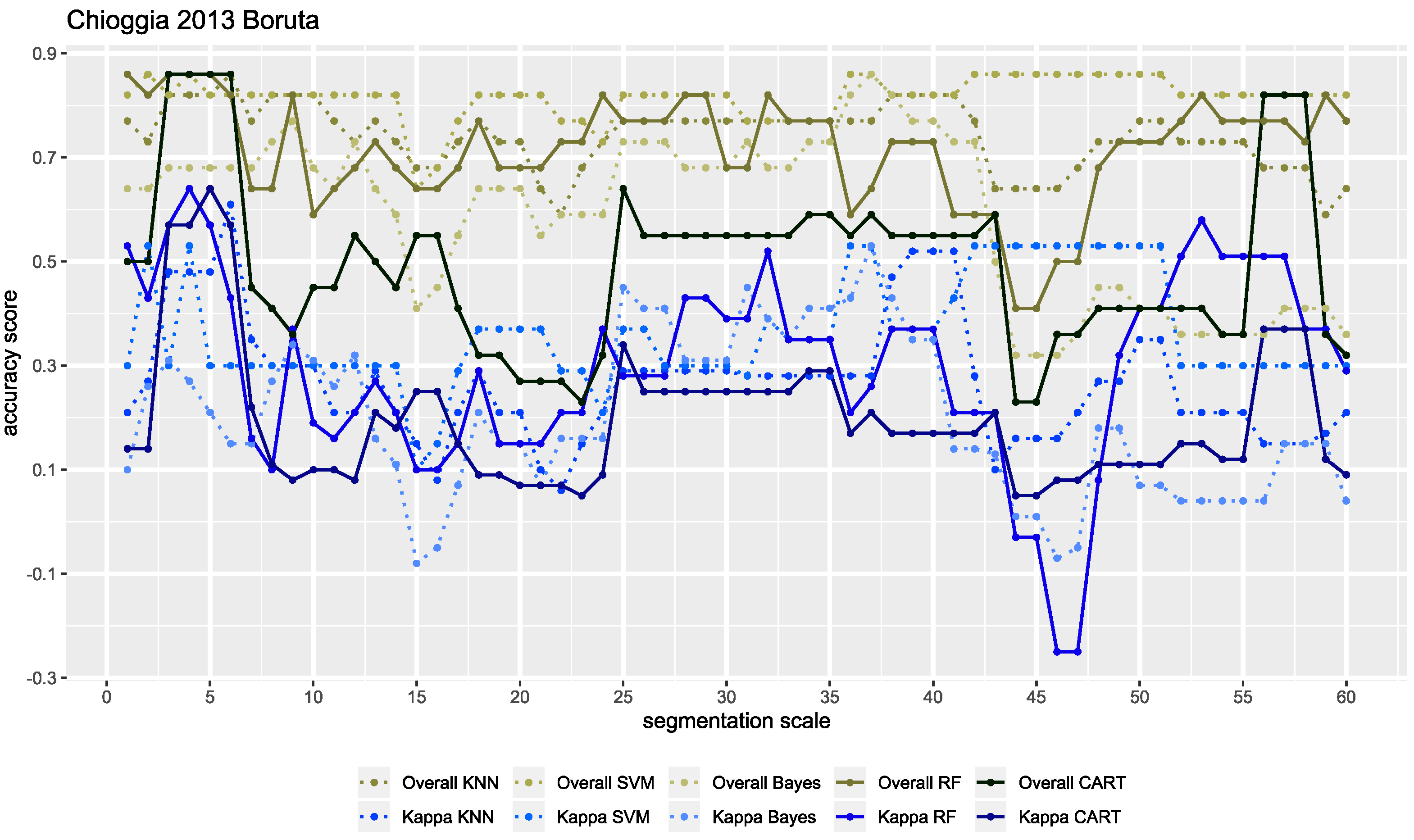
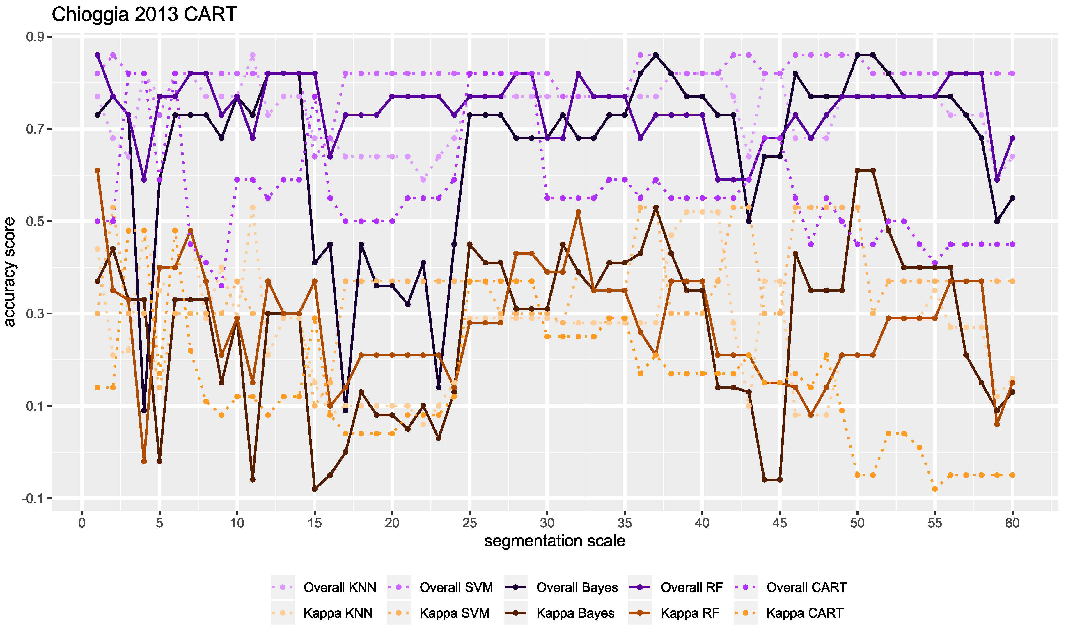
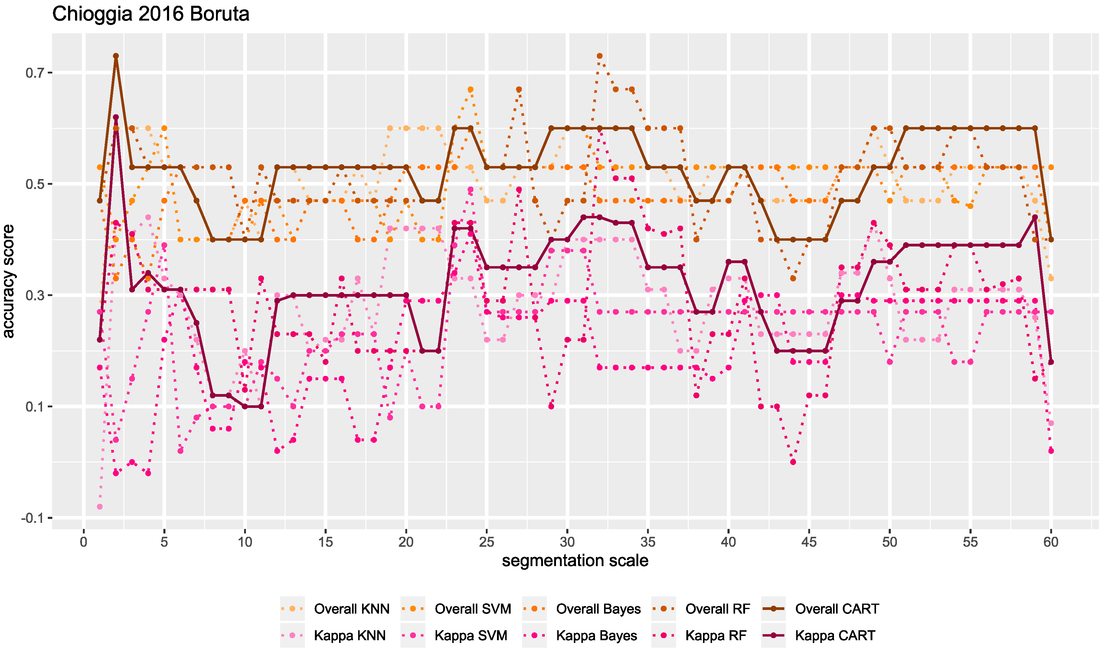
3.4. Image Segmentation, Classification, and Accuracy Assessment

The tested multiresolution segmentation scale from 1 to 60 gave an average object size of approximately 0.55 to 3258.87 m². Segmentation results for each scale were classified by four to five classifiers, giving up to 300 results for each dataset. Each classifier was trained using two sets of important features (selected by the Boruta or CART algorithm). Overall, we obtained 1124 classification results, from which we selected the outcomes with the highest accuracy assessment statistics. The highest scores were achieved by the CART, RF, and Bayes classifiers. As many results had similar high overall accuracy scores, we also selected the results based on the kappa accuracy outcomes. Summary line plots of the overall and kappa statistics for all classifiers and multiresolution segmentation scales are shown in Figure A1, Figure A2, Figure A3 and Figure A4. They represent dependencies between multiresolution segmentation scales and used classifiers vs. accuracy assessment scores. We used the graphs to evaluate the models and select the results with the highest performance, based on their accuracy.

The dependency between multiresolution segmentation scale and classification accuracy, determined with features selected by the Boruta algorithm for the Chioggia 2013 dataset, indicated that two classifiers had the best accuracy, RF and CART, for segmentation scales 4 and 5, respectively (Figure A1). The highest overall accuracy reached 0.86, with kappa = 0.64. Linear dependence between the overall and kappa accuracy was between 0.85 and 0.92 for the RF and CART classifiers. The relationship between accuracy and the object-based segmentation scale for the Chioggia 2013 dataset using the CART feature-selection algorithm is shown in Figure A2. Two classifier algorithms (RF, Bayes) performed with the highest accuracy at three multiresolution segmentation scales, 1, 50, and 51. Overall accuracy was 0.86, with kappa = 0.61. The charts show the scale variability for different classifiers. Linear dependence between the overall and kappa accuracy was average, at 0.65 and 0.66 for the RF and Bayes classifiers, respectively.

Figure A3 and Figure A4 refer to the dependency between scale and accuracy assessment for the Chioggia 2016 dataset, in relation to the feature selection technique. Due to the separation of more classes, in general, the accuracy scores were worse than that for the 2013 dataset. Charts of classifier accuracy showed low to high variability versus multiresolution segmentation scale. Independent of the feature selection method used, the best accuracy outcomes were obtained with the CART classifier, reaching 0.73 for overall accuracy and 0.62 for the kappa index of agreement. With the Boruta feature selection method, the highest accuracy was achieved for multiresolution segmentation scale 2, and with CART, the highest accuracy was obtained for scale 23 (Figure A3 and Figure A4). For both 2016 datasets, Pearson’s linear correlation coefficient between kappa and the overall accuracy for the best charts was very high, from 0.95 to 0.99.

From all outcomes with the highest accuracy, we selected the following models—(A) Chioggia 2013 dataset, Boruta feature selection, RF classifier, scale 4 of multiresolution segmentation; (B) Chioggia 2013 dataset, CART feature selection, Bayes classifier, scale 50 of multiresolution segmentation; (C) Chioggia 2016 dataset, CART feature selection, CART classifier, scale 23 of multiresolution segmentation; and (D) Chioggia 2016 dataset, Boruta feature selection, RF classifier, scale 32 of multiresolution segmentation. Sediment composition maps for the four considered models are presented in Figure 5.

Detailed error matrices for the models with the highest accuracy are presented in

Table 3. Error matrices with accuracy assessment for all Chioggia datasets: (A) Chioggia 2013 dataset, Boruta feature selection, RF classifier, scale 4 of multiresolution segmentation; (B) Chioggia 2013 dataset, CART feature selection, Bayes classifier, scale 50 of multiresolution segmentation; (C) Chioggia 2016 dataset, CART feature selection, CART classifier, scale 23 of multiresolution segmentation; and (D) Chioggia 2016 dataset, Boruta feature selection, RF classifier, scale 32 of multiresolution segmentation.

A		Reference					B		Reference
		M + SM	S + MS	CS	Sum				M + SM	S + MS	CS	Sum
Prediction	M + SM	1	1	0	2		Prediction	M + SM	1	1	0	2
	S + MS	1	16	0	17			S + MS	2	16	0	18
	CS	1	0	2	3			CS	0	0	2	2
	Sum	3	17	2	22			Sum	3	17	2	22
	Producer’s	0.33	0.94	1.00				Producer’s	0.33	0.94	1.00
	User’s	0.50	0.94	0.67				User’s	0.50	0.89	1.00
	Overall accuracy	0.86						Overall accuracy	0.86
	Kappa	0.64						Kappa	0.61
C		Reference					D		Reference
		CS	MIX	M + SM	S + MS	Sum			CS	MIX	M + SM	S + MS	Sum
Prediction	CS	6	1	1	0	8	Prediction	CS	5	1	0	1	7
	MIX	0	2	0	1	3		MIX	1	2	1	0	4
	M + SM	0	0	1	0	1		M + SM	0	0	2	0	2
	S + MS	0	0	1	2	3		S + MS	0	0	0	2	2
	Sum	6	3	3	3	15		Sum	6	3	3	3	15
	Producer’s	1.00	0.67	0.33	0.67			Producer’s	0.83	0.67	0.67	0.67
	User’s	0.75	0.67	1.00	0.67			User’s	0.71	0.50	1.00	1.00
	Overall accuracy	0.73						Overall accuracy	0.73
	Kappa	0.62						Kappa	0.62

, showing a good and very good overall and kappa accuracy. The results of both 2013 datasets indicated that the S + MS and CS classes had good and very good accuracy, up to 1.00, for all statistics of CS with CART. The remaining class of M + SM had fair to moderate statistics per class, depending on the accuracy statistics. The last two confusion matrices refer to the Chioggia 2016 dataset results. The dataset with the CART feature selection method represented ideal accuracy of the CS class (1.00), good performance for the S + MS and MIX classes, and fair to moderate accuracy of the M + SM class (depending on the accuracy statistics). The results of the Boruta feature-selection algorithm with the RF classifier showed that all sediment types were classified with very similar, moderate to good accuracy per class (depending on specific accuracy statistics; see Table 3).

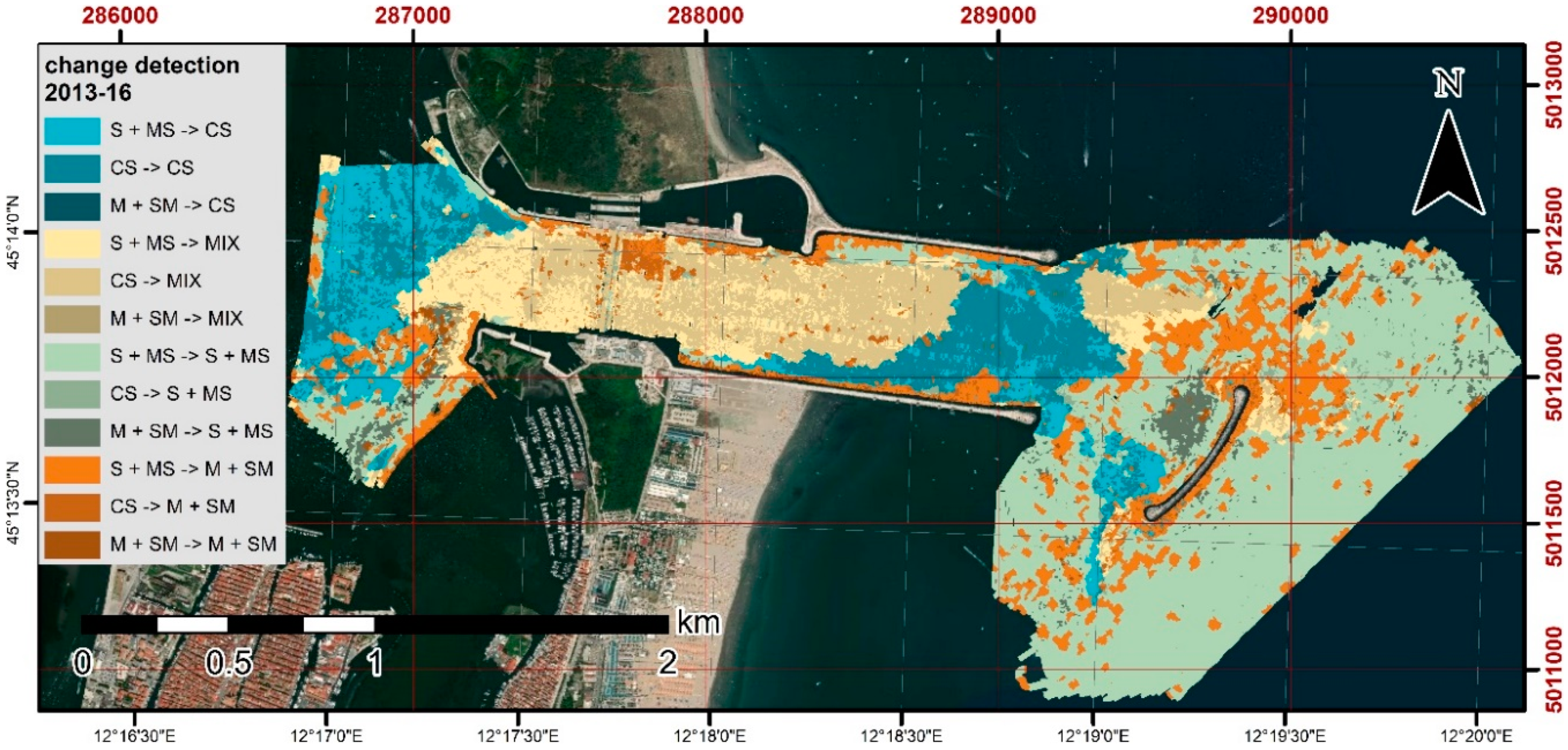
3.5. Change Detection

Models A and C were considered for further change detection analysis. The transition matrix of selected classification results is presented in

Table 4. Change detection transition matrix of habitat classes in Chioggia 2013 and 2016 AOIs. Bold numbers refer to the persistence of classes.

	Habitat Class	2016
		CS	MIX	M + SM	S + MS	Total 2013
2013	CS	10.07	12.15	1.74	1.00	24.97
	M + SM	0.08	0.30	0.91	2.50	3.78
	S + MS	9.28	8.42	14.08	39.46	71.25
	Total 2016	19.44	20.87	16.72	42.97	100.00

. Parts of the area covered by specific sediment classes are expressed as percentages of the whole study area. As the number of sediment types was not the same for both surveys, the matrix was not symmetrical. For this reason, the MIX class did not have any persistent statistics. Table 4 indicates that the largest area for both surveys was covered by the S + MS type. Similarly, in both cases, the smallest area was occupied by M + SM. The CS and MIX classes covered moderate parts of the whole area; the latter was present only in the 2016 dataset. Similar to Table 4, all results in

Table 5. Change detection statistics for the habitat classes of the Chioggia 2013 and 2016 study areas.

Class	Total 2013	Total 2016	Gain	Loss	Total Change	Swap (Location)	Net (Quantity)	G/p	L/p	N/p
CS	24.97	19.44	9.37	14.90	24.26	18.73	5.53	0.93	1.48	−0.55
MX	-	20.87	20.87	0	20.87	0.00	20.87	-	-	-
M_SM	3.78	16.72	15.81	2.88	18.69	5.76	12.94	17.47	3.18	14.29
S_MS	71.25	42.97	3.51	31.78	35.29	7.01	−28.28	0.09	0.81	−0.72
Total	100.00	100.00	49.56	49.56	99.12	31.50	67.61

are presented in percentages. As the high gain statistic of the MIX type (related to its absence in 2013), the M + SM and CS classes also had high-gain coefficients. High loss was observed in S + MS and CS. In general, considering the total gain and loss statistics, almost 50% of the area increased or decreased, which gave nearly 100% of the total change. From the spatial point of view, the CS class had the largest swap between the analyzed time steps, whereas two other classes (except the MIX class) had a moderate swap. It seemed that the quantity of S + MS decreased almost 30%, in comparison to the smaller decrease of CS, whereas MIX and M + SM increased almost 21%. The statistics for the last three ratios showed that the CS and S + MS classes were generally stable. The ratio of L/p for CS indicated a loss tendency for this class. The statistics for M + SM showed a highly positive change tendency and a probability of gain, as well as a high loss probability, so this class was the most inconsistent of all. A map of change detection for the 2013 and 2016 datasets is presented in Figure 6.

According to Rattray et al. [10], accuracy assessment of change detection could be estimated by multiplying their results for the whole time-series. Therefore, the overall accuracy of change detection was 63% and the kappa coefficient was 0.40, meaning that 40% of the change did not occur by chance.

4. Discussion

Change detection statistics presented in Table 5 suggests a very high dynamic of sediment substrates located in the Chioggia inlet, which is in line with other results found in the literature concerning bathymetry changes in 2002–2013 [37], and in 2004–2014 in the neighboring Lido inlet, located in the north of the Venice Lagoon [15].

Sediment maps of the Chioggia dataset from the 2013 survey were previously analyzed using two methods of pixel-based classification, maximum likelihood classifier (MLC; supervised), and Jenks (unsupervised) [37,82]. These classifications separated the ground truth sediment samples for four categories—sandy gravel + gravelly sand; sandy gravelly sand; sand; and slightly gravelly muddy sand + muddy sand + slightly gravelly sandy mud. Overall accuracy for MLC was 0.71, whereas for Jenks the natural breaks optimization reached 0.75 [37,82]. In this study, we used sediment composition models based on the EUNIS sediment classification with different ground truth categories. The EUNIS scheme of marine sediment classification was applied in several habitat-mapping studies [11,68,83]. In these studies, the authors emphasized on the simplicity and ease of interpreting ground truth data, based on this scheme [83]. In our study, the EUNIS classification was enough to separate the MBES backscatter characteristics. However, a different classification scheme should be applied for a more complete characterization of the substrate [31,37,82].

Time series of sediment composition in this study were the result of comparing two supervised classifications, based on separate ground truth sampling for each survey. A similar approach was presented by Rattray et al. [10], who determined four classes of benthic habitats, based on separate ground truth campaigns. In this study, we focused on evaluating a change-detection sediment composition map, using the OBIA approach and comparing multiple classifiers.

4.1. Performance of Relevant Classifiers

Among others, the CART classifier was applied in a few mapping studies of seafloor sediment [66,84]. Along with CART, other decision trees were also applied in various marine habitat-mapping studies [22,23,85,86,87]. The highest overall accuracy scores of some of these studies ranged from 0.8 [85,86] to 0.88 [66]. Compared to other studies, the performance of the CART classifier for both Chioggia areas was good and fit well with the models concerning the decision trees.

The performance of the RF classifier was better between the two models selected in this study. In recent marine habitat-mapping studies, RF became a very promising semi-automated method of habitat classification [8]. Compared to other classifiers, the accuracy of RF was often among the highest [22,68,88]. In terms of accuracy statistics, the results presented in this study were approximately the average of other results in the literature (see, e.g., [18,22,68]).

One selected model (Chioggia 2013 with CART) represented the high usefulness of the Bayes classifier algorithm. A comparison with other habitat-mapping studies, based on an image-processing approach indicated that the Bayes classifier applied in [23] was determined to have the best performance. In that study, it reached an overall accuracy of 0.8 and a kappa coefficient of 0.5. As a signal processing approach, the Bayes classifier was used in another study, but the accuracy assessment of the classification results was not described using any metric [89].

4.2. Geological Interpretation of Results

Based on bathymetric and sediment distribution changes, the microtidal sedimentary environment of the Chioggia region was described. Two sedimentary environments were determined in the region characterized by varying energy, corresponding to the hydrodynamic regime of the area proposed in [37]. The first one comprised the channel connecting the lagoon with the sea, where the cross-section and bottom relief were anthropogenically modified since 2003, when the MoSE project was launched [36]. This part was dominated by very coarse-grained sand, with an average content of silt-clay fractions, not exceeding 4%. The other environment was located at the inlet front, where the grain diameter of the sediment clearly decreased (turning into fine-grained sand and medium-grained silt). The enrichment with fine fractions was considerably greater and spatially diverse. The content of silt-clay fractions reached about 75% on the landward side of the breakwater, and about 12% on the seaward side. The increased fractions in the first case were the result of microcirculation between the breakwater and the Chioggia inlet, which could be a trap for fine fractions transported in suspension [34]. The sorting of sediment in both environments was poor, which might be related to the highly variable energy of the sedimentary environment. The relationship was also confirmed by mostly low values of kurtosis (platykurtic grain-size distribution).

In addition to changes in the depositional environment along the channel, the sedimentary regime also changed in the profile crossing of the axis of the channel (Figure 7). Grain size changes were related to the channel’s hydrodynamics. Sediment became finer from north to south, sorting increased, and the kurtosis values were higher (Figure 8), which corresponded to the smaller energy diversity of the sedimentary environment. The reduced energy in the southern area might be related to rip-rap debris, which was asymmetrically distributed along the channel in the shape of a “trail” that gradually covered the bottom from the southern jetty to the central and the northern part of the channel, moving towards the sea [37]. The presence of the debris controlled the accumulation of sand, which led to the deposition of sediment in the form of large dunes at the southern jetty (Figure 7).

The human impact associated with the construction of the MoSE barriers in the Chioggia region had affected the hydrodynamic regime of the inlet. We observed activities such as reducing the width of the Chioggia inlet for the MoSE infrastructure, building rip-rap revetments on the channel bottom, and constructing a breakwater in front of inlet. These modified the length and direction of the outflow jet patterns of currents around the inlet [34,37], which was reflected in the morphological and sedimentary changes of this area.

4.3. Suggestions for Future Research

The results presented in this work were produced using OBIA, assuming a supervised classification. Especially in terms of further change detection studies elsewhere, modern MBES calibrated for acoustic backscatter, potentially allow knowledge-based unsupervised classification after single ground truth identification of benthic habitats. It might be important especially because of cost restrictions or specific survey plans, where ground truth sampling of the whole time-series might not be possible. Such approaches for time-series of MBES measurements were recently applied using supervised and unsupervised classification techniques, based on single ground truth campaigns. For example, the change detection study of Montereale-Gavazzi et al. [11] used K-means unsupervised classification to find the optimal solution for the results of multiple MBES time-series, based on the single results of RF classification. In this case, the authors kept rigorous standards of the MBES backscatter data acquisition in natural reference areas, resulting in low backscatter fluctuations through the whole time-series of the MBES. It allowed them to compare average backscatter values from one survey to another. The recent study of Gaida et al. [13] showed a promising application of unsupervised Bayesian classification to time-series of MBES measurements. For comparison, OBIA was not designed to perform typical unsupervised classification, based on backscatter intensity values. However, it benefitted from so-called knowledge-based classification, allowing the development of rule sets, assigning objects based on their spectral, contextual, textural, and shape properties [90]. It seems that this provided a great opportunity for the classification of calibrated backscatter datasets, while being much more complicated than the pixel-based approach.

Interestingly, the best accuracy results for both Chioggia surveys were achieved using the Boruta feature-selection algorithm, which indicated two of the highest derivatives for classification—backscatter and GLCM mean. Recent research suggests that the GLCM mean showed good agreement with sediment classes generated using angular range analysis (ARA) [91]. Generating ARA sediment maps on the Chioggia datasets and comparing them with just created habitat maps could contribute to further conclusions between image and signal processing methods.

The set of 25 secondary features used in this study fit well in the current predictive habitat mapping literature [18,92]. According to Ierodiaconou et al. [18], the combination of pixel- and object-based secondary features is promising and could give better results than when either were used separately. In order to select the features properly, we compared two feature-selection algorithms. Further study might include arranging other feature selection methods and extracting larger feature sets, including, e.g., spectral features of rough seafloor surface or additional backscatter and oceanographic variables. Among others, there are useful backscatter features mentioned in the literature, such as spatial autocorrelation [23,68,93], hue, saturation, intensity [86,87,94,95], ARA [22,85,94], and Q-values [2,96,97]. Another study suggested calculating maximum orbital velocity as an oceanographic variable [95].

5. Conclusions

This study concerned the importance of research approaches and methodical tools that could be used for marine environment assessment of various scales.

Repeated mapping of the Chioggia inlet allowed us to determine the seafloor sediment properties and follow their temporal variability. This monitoring activity was crucial, considering that MoSE barriers are currently in operation, given the high degree of hydrodynamic variation and strong anthropogenic pressure and the impact on seabed sediment transport.

The overall achievement of this work was the development of an innovative method of seabed habitat-classification, based on automated OBIA analysis and supervised classifiers. This method was applied and tested in the tidal environment of the Lagoon of Venice. The analysis included extracting a large number of MBES bathymetry and backscatter features. They were calculated using pixel- and object-based methods. An objective feature-selection approach was used, applying and comparing the CART and Boruta algorithms. Along with backscatter intensity, different secondary features were selected, depending on the dataset. For the Chioggia AOI, secondary features based on the GLCM texture derivatives were the most relevant for classification. Bayes, CART, and RF classifiers also showed good performance, compared to other studies.

The study investigated how classification accuracy could be affected by the scale of the object-based segmentation. The size of image objects was estimated using OBIA multi-scale accuracy assessment, related to a very large set of multiresolution segmentation results. Dependencies between the scales of multiresolution segmentation and accuracy assessment showed that using the proper scale of object-based segmentation made it possible to reach high accuracy in classification. However, the choice of scale should be properly tuned and tested.

Applying the classification method at the proper scale allowed us to observe the habitat changes in the tidal inlet of the Venice Lagoon, showing that the sediment substrates in the Chioggia inlet were subjected to very dynamic changes. In general, during the study period, the area was enriched in mixed and muddy sediments and depleted in sandy deposits.

The methodological approaches described here could be easily applied to other geographical areas and scales, in both shallow and deep marine environments. The main requirement was good-quality hydroacoustic and ground truth data to support the monitoring and management of the marine environment. The procedures developed in this study might help to establish a standard tool for Descriptor 6 of the Marine Strategy Framework Directive, concerning the integrity of the seafloor.

References

1. Harris, P.T.; Baker, E.K. Why Map Benthic Habitats? In Seafloor Geomorphology as Benthic Habitat; Harris, P.T., Baker, E.K., Eds.; Elsevier: London, UK, 2012; pp. 3–22. [Google Scholar]
2. McGonigle, C.; Brown, C.; Quinn, R.; Grabowski, J. Evaluation of image-based multibeam sonar backscatter classification for benthic habitat discrimination and mapping at Stanton Banks, UK. Estuar. Coast. Shelf Sci. 2009, 81, 423–437. [Google Scholar] [CrossRef]
3. Thorsnes, T.; Bjarnadóttir, L.R.; Jarna, A.; Baeten, N.; Scott, G.; Guinan, J.; Monteys, X.; Dove, D.; Green, S.; Gafeira, J.; et al. National Programmes: Geomorphological Mapping at Multiple Scales for Multiple Purposes. In Submarine Geomorphology; Micallef, A., Krastel, S., Savini, A., Eds.; Springer International Publishing: Cham, Germany, 2018; pp. 535–552. [Google Scholar] [CrossRef]
4. Picard, K.; Whiteway, T.; Leplastrier, A.; Team, A. AusSeabed: Collaborating to Maximise Australian Seabed Mapping Efforts. In AGU Fall Meeting Abstracts; American Geophysical Union: Washington, DC, USA, 2018. [Google Scholar]
5. Madricardo, F.; Foglini, F.; Kruss, A.; Ferrarin, C.; Pizzeghello, N.M.; Murri, C.; Rossi, M.; Bajo, M.; Bellafiore, D.; Campiani, E.; et al. High resolution multibeam and hydrodynamic datasets of tidal channels and inlets of the Venice Lagoon. Sci. Data 2017, 4, 170121. [Google Scholar] [CrossRef] [Green Version]
6. Brown, C.J.; Smith, S.J.; Lawton, P.; Anderson, J.T. Benthic habitat mapping: A review of progress towards improved understanding of the spatial ecology of the seafloor using acoustic techniques. Estuar. Coast. Shelf Sci. 2011, 92, 502–520. [Google Scholar] [CrossRef]
7. Lucieer, V.; Lucieer, A. Fuzzy clustering for seafloor classification. Mar. Geol. 2009, 264, 230–241. [Google Scholar] [CrossRef]
8. Lucieer, V.; Hill, N.A.; Barrett, N.S.; Nichol, S. Do marine substrates ‘look’ and ‘sound’ the same? Supervised classification of multibeam acoustic data using autonomous underwater vehicle images. Estuar. Coast. Shelf Sci. 2013, 117, 94–106. [Google Scholar] [CrossRef]
9. Lecours, V. On the Use of Maps and Models in Conservation and Resource Management (Warning: Results May Vary). Front. Mar. Sci. 2017, 4, 288. [Google Scholar] [CrossRef] [Green Version]
10. Rattray, A.; Ierodiaconou, D.; Monk, J.; Versace, V.L.; Laurenson, L.J.B. Detecting patterns of change in benthic habitats by acoustic remote sensing. Mar. Ecol. Prog. Ser. 2013, 477, 1–13. [Google Scholar] [CrossRef] [Green Version]
11. Montereale-Gavazzi, G.; Roche, M.; Lurton, X.; Degrendele, K.; Terseleer, N.; Van Lancker, V. Seafloor change detection using multibeam echosounder backscatter: Case study on the Belgian part of the North Sea. Mar. Geophys. Res. 2018, 39, 229–247. [Google Scholar] [CrossRef]
12. Fezzani, R.; Berger, L. Analysis of calibrated seafloor backscatter for habitat classification methodology and case study of 158 spots in the Bay of Biscay and Celtic Sea. Mar. Geophys. Res. 2018, 39, 169–181. [Google Scholar] [CrossRef] [Green Version]
13. Gaida, T.C.; van Dijk, T.A.G.P.; Snellen, M.; Vermaas, T.; Mesdag, C.; Simons, D.G. Monitoring underwater nourishments using multibeam bathymetric and backscatter time series. Coast. Eng. 2020, 158, 103666. [Google Scholar] [CrossRef]
14. Montereale-Gavazzi, G.; Roche, M.; Degrendele, K.; Lurton, X.; Terseleer, N.; Baeye, M.; Francken, F.; Van Lancker, V. Insights into the Short-Term Tidal Variability of Multibeam Backscatter from Field Experiments on Different Seafloor Types. Geosciences 2019, 9, 34. [Google Scholar] [CrossRef]
15. Toso, C.; Madricardo, F.; Molinaroli, E.; Fogarin, S.; Kruss, A.; Petrizzo, A.; Pizzeghello, N.M.; Sinapi, L.; Trincardi, F. Tidal inlet seafloor changes induced by recently built hard structures. PLoS ONE 2019, 14, e0223240. [Google Scholar] [CrossRef] [PubMed]
16. Hughes Clarke, J.E. Multibeam Echosounders. In Submarine Geomorphology; Micallef, A., Krastel, S., Savini, A., Eds.; Springer International Publishing: Cham, Germany, 2018; pp. 25–41. [Google Scholar] [CrossRef]
17. Wendelboe, G. Backscattering from a sandy seabed measured by a calibrated multibeam echosounder in the 190–400 kHz frequency range. Mar. Geophys. Res. 2018, 39, 105–120. [Google Scholar] [CrossRef]
18. Ierodiaconou, D.; Schimel, A.C.G.; Kennedy, D.; Monk, J.; Gaylard, G.; Young, M.; Diesing, M.; Rattray, A. Combining pixel and object based image analysis of ultra-high resolution multibeam bathymetry and backscatter for habitat mapping in shallow marine waters. Mar. Geophys. Res. 2018, 39, 271–288. [Google Scholar] [CrossRef]
19. Lacharité, M.; Brown, C.J.; Gazzola, V. Multisource multibeam backscatter data: Developing a strategy for the production of benthic habitat maps using semi-automated seafloor classification methods. Mar. Geophys. Res. 2018, 39, 307–322. [Google Scholar] [CrossRef]
20. Innangi, S.; Tonielli, R.; Romagnoli, C.; Budillon, F.; Di Martino, G.; Innangi, M.; Laterza, R.; Le Bas, T.; Lo Iacono, C. Seabed mapping in the Pelagie Islands marine protected area (Sicily Channel, southern Mediterranean) using Remote Sensing Object Based Image Analysis (RSOBIA). Mar. Geophys. Res. 2019, 40, 333–355. [Google Scholar] [CrossRef] [Green Version]
21. Lucieer, V.; Lamarche, G. Unsupervised fuzzy classification and object-based image analysis of multibeam data to map deep water substrates, Cook Strait, New Zealand. Cont. Shelf Res. 2011, 31, 1236–1247. [Google Scholar] [CrossRef]
22. Hasan, R.; Ierodiaconou, D.; Monk, J. Evaluation of Four Supervised Learning Methods for Benthic Habitat Mapping Using Backscatter from Multi-Beam Sonar. Remote Sens. 2012, 4, 3427–3443. [Google Scholar] [CrossRef] [Green Version]
23. Stephens, D.; Diesing, M. A comparison of supervised classification methods for the prediction of substrate type using multibeam acoustic and legacy grain-size data. PLoS ONE 2014, 9, e93950. [Google Scholar] [CrossRef]
24. Mitchell, P.J.; Downie, A.-L.; Diesing, M. How good is my map? A tool for semi-automated thematic mapping and spatially explicit confidence assessment. Environ. Model. Softw. 2018, 108, 111–122. [Google Scholar] [CrossRef]
25. Misiuk, B.; Diesing, M.; Aitken, A.; Brown, C.J.; Edinger, E.N.; Bell, T. A Spatially Explicit Comparison of Quantitative and Categorical Modelling Approaches for Mapping Seabed Sediments Using Random Forest. Geosciences 2019, 9, 254. [Google Scholar] [CrossRef] [Green Version]
26. Wynn, R.B.; Huvenne, V.A.I.; Le Bas, T.P.; Murton, B.J.; Connelly, D.P.; Bett, B.J.; Ruhl, H.A.; Morris, K.J.; Peakall, J.; Parsons, D.R.; et al. Autonomous Underwater Vehicles (AUVs): Their past, present and future contributions to the advancement of marine geoscience. Mar. Geol. 2014, 352, 451–468. [Google Scholar] [CrossRef] [Green Version]
27. Jones, D.O.B.; Gates, A.R.; Huvenne, V.A.I.; Phillips, A.B.; Bett, B.J. Autonomous marine environmental monitoring: Application in decommissioned oil fields. Sci. Total Environ. 2019, 668, 835–853. [Google Scholar] [CrossRef]
28. Umgiesser, G.; Canu, D.M.; Cucco, A.; Solidoro, C. A finite element model for the Venice Lagoon. Development, set up, calibration and validation. J. Mar. Syst. 2004, 51, 123–145. [Google Scholar] [CrossRef]
29. Molinaroli, E.; Guerzoni, S.; Sarretta, A.; Masiol, M.; Pistolato, M. Thirty-year changes (1970 to 2000) in bathymetry and sediment texture recorded in the Lagoon of Venice sub-basins, Italy. Mar. Geol. 2009, 258, 115–125. [Google Scholar] [CrossRef] [Green Version]
30. Albani, A.D.; Donnici, S.; Serandrei-Barbero, R.; Rickwood, P.C. Seabed sediments and foraminifera over the Lido Inlet: Comparison between 1983 and 2006 distribution patterns. Cont. Shelf Res. 2010, 30, 847–858. [Google Scholar] [CrossRef]
31. Madricardo, F.; Foglini, F.; Campiani, E.; Grande, V.; Catenacci, E.; Petrizzo, A.; Kruss, A.; Toso, C.; Trincardi, F. Assessing the human footprint on the sea-floor of coastal systems: The case of the Venice Lagoon, Italy. Sci. Rep. 2019, 9, 6615. [Google Scholar] [CrossRef]
32. Trincardi, F.; Barbanti, A.; Bastianini, M.; Benetazzo, A.; Cavaleri, L.; Chiggiato, J.; Papa, A.; Pomaro, A.; Sclavo, M.; Tosi, L.; et al. The 1966 Flooding of Venice: What Time Taught Us for the Future. Oceanography 2016, 29, 178–186. [Google Scholar] [CrossRef] [Green Version]
33. The ISMAR Team: Cavaleri, L.; Bajo, M.; Barbariol, F.; Bastianini, M.; Benetazzo, A.; Bertotti, L.; Chiggiato, J.; Ferrarin, C.; Trincardi, F.; Umgiesser, G. The 2019 flooding of Venice and Its Implications for Future Predictions. Oceanography 2020, 33, 42–49. [Google Scholar] [CrossRef] [Green Version]
34. Ghezzo, M.; Guerzoni, S.; Cucco, A.; Umgiesser, G. Changes in Venice Lagoon dynamics due to construction of mobile barriers. Coast. Eng. 2010, 57, 694–708. [Google Scholar] [CrossRef] [Green Version]
35. Umgiesser, G.; Matticchio, B. Simulating the mobile barrier (MOSE) operation in the Venice Lagoon, Italy: Global sea level rise and its implication for navigation. Ocean Dyn. 2006, 56, 320–332. [Google Scholar] [CrossRef]
36. Villatoro, M.M.; Amos, C.L.; Umgiesser, G.; Ferrarin, C.; Zaggia, L.; Thompson, C.E.L.; Are, D. Sand transport measurements in Chioggia inlet, Venice lagoon: Theory versus observations. Cont. Shelf Res. 2010, 30, 1000–1018. [Google Scholar] [CrossRef]
37. Fogarin, S.; Madricardo, F.; Zaggia, L.; Sigovini, M.; Montereale-Gavazzi, G.; Kruss, A.; Lorenzetti, G.; Manfé, G.; Petrizzo, A.; Molinaroli, E.; et al. Tidal inlets in the Anthropocene: Geomorphology and benthic habitats of the Chioggia inlet, Venice Lagoon (Italy). Earth Surf. Process. Landf. 2019, 44, 2297–2315. [Google Scholar] [CrossRef]
38. Donda, F.; Brancolini, G.; Tosi, L.; Kovačević, V.; Baradello, L.; Gačić, M.; Rizzetto, F. The ebb-tidal delta of the Venice Lagoon, Italy. Holocene 2008, 18, 267–278. [Google Scholar] [CrossRef]
39. Zecchin, M.; Baradello, L.; Brancolini, G.; Donda, F.; Rizzetto, F.; Tosi, L. Sequence stratigraphy based on high-resolution seismic profiles in the late Pleistocene and Holocene deposits of the Venice area. Mar. Geol. 2008, 253, 185–198. [Google Scholar] [CrossRef]
40. Wentworth, C.K. A Scale of Grade and Class Terms for Clastic Sediments. J. Geol. 1922, 30, 377–392. [Google Scholar] [CrossRef]
41. Folk, R.L. The distinction between grain size and mineral composition in sedimentary rock nomenclature. J. Geol. 1954, 62, 344–359. [Google Scholar] [CrossRef]
42. Folk, R.L. A Review of Grain-Size Parameters. Sedimentology 1966, 6, 73–93. [Google Scholar] [CrossRef]
43. Folk, R.L.; Ward, W.C. Brazos River bar [Texas]; a study in the significance of grain size parameters. J. Sediment. Res. 1957, 27, 3–26. [Google Scholar] [CrossRef]
44. Fonseca, L.; Calder, B. Geocoder: A Efficient Backscatter Map Constructor; Hydrographic Society of America: San Diego CA, USA, 2015. [Google Scholar]
45. Beaudoin, J.; Hughes Clarke, J.E.; Van Den Ameele, E.J.; Gardner, J.V. Geometric and Radiometric Correction of Multibeam Backscatter Derived from Reson 8181 Systems. In Proceedings of the Canadian Hydrographic Conference (CHC), Toronto, ON, Canada, 28–31 May 2008. [Google Scholar]
46. Fonseca, L.; Brown, C.; Calder, B.; Mayer, L.; Rzhanov, Y. Angular range analysis of acoustic themes from Stanton Banks Ireland: A link between visual interpretation and multibeam echosounder angular signatures. Appl. Acoust. 2009, 70, 1298–1304. [Google Scholar] [CrossRef]
47. Walbridge, S.; Slocum, N.; Pobuda, M.; Wright, D. Unified Geomorphological Analysis Workflows with Benthic Terrain Modeler. Geosciences 2018, 8, 94. [Google Scholar] [CrossRef] [Green Version]
48. Burrough, P.A.; McDonell, R.A. Principles of Geographical Information Systems; Oxford University Press: New York, NY, USA, 1998. [Google Scholar]
49. Roberts, D.W. Ordination on the basis of fuzzy set theory. Vegetatio 1986, 66, 123–131. [Google Scholar] [CrossRef]
50. Zevenbergen, L.W.; Thorne, C.R. Quantitative analysis of land surface topography. Earth Surf. Process. Landf. 1987, 12, 47–56. [Google Scholar] [CrossRef]
51. Hobson, R.D. Surface roughness in topography: Quantitative approach. In Spatial Analysis in Geomorphology; Chorley, R.J., Ed.; Harper and Row: New York, NY, USA, 1972; pp. 221–245. [Google Scholar]
52. Sappington, J.M.; Longshore, K.M.; Thompson, D.B. Quantifying Landscape Ruggedness for Animal Habitat Analysis: A Case Study Using Bighorn Sheep in the Mojave Desert. J. Wildl. Manag. 2007, 71, 1419–1426. [Google Scholar] [CrossRef]
53. Wilson, M.F.J.; O’Connell, B.; Brown, C.; Guinan, J.C.; Grehan, A.J. Multiscale Terrain Analysis of Multibeam Bathymetry Data for Habitat Mapping on the Continental Slope. Mar. Geod. 2007, 30, 3–35. [Google Scholar] [CrossRef] [Green Version]
54. Haralick, R.M.; Shanmugam, K.; Dinstein, I.H. Textural Features for Image Classification. IEEE Trans. Syst. ManCybern. 1973, SMC-3, 610–621. [Google Scholar] [CrossRef] [Green Version]
55. Hall-Beyer, M. GLCM Texture: A Tutorial. National Council on Geographic Information and Analysis Remote Sensing Core Curriculum. 2007. Available online: https://prism.ucalgary.ca/handle/1880/51900 (accessed on 30 June 2020).
56. van der Sanden, J.J.; Hoekman, D.H. Review of relationships between grey-tone co-occurrence, semivariance, and autocorrelation based image texture analysis approaches. Can. J. Remote Sens. 2014, 31, 207–213. [Google Scholar] [CrossRef]
57. Breiman, L.; Friedman, J.H.; Olshen, R.A.; Stone, C.J. Classification and Regression Trees; Wadsworth: Belmont, UK, 1984. [Google Scholar]
58. Guyon, I.; Elisseeff, A. An introduction to Variable and Feature Selection. J. Mach. Learn. Res. 2003, 3, 1157–1182. [Google Scholar]
59. Saeys, Y.; Inza, I.; Larranaga, P. A review of feature selection techniques in bioinformatics. Bioinformatics 2007, 23, 2507–2517. [Google Scholar] [CrossRef] [PubMed] [Green Version]
60. Kursa, M.B.; Rudnicki, W.R. Feature Selection with the Boruta Package. J. Stat. Softw. 2010, 36. [Google Scholar] [CrossRef] [Green Version]
61. Kursa, M.B.; Rudnicki, W.R. Package ‘Boruta’. Wrapper Algorithm for All Relevant Feature Selection. 2016. Available online: https://m2.icm.edu.pl/boruta/ (accessed on 19 April 2017).
62. Bivand, R.; Keitt, T.; Rowlingson, B.; Pebesma, E.; Sumner, M.; Hijmans, R.; Rouault, E. Package ‘rgdal’. Bindings for the Geospatial Data Abstraction Library. Available online: https://cran.r-project.org/web/packages/rgdal/index.html (accessed on 15 October 2017).
63. Hay, G.J.; Castilla, G. Object-Based Image Analysis: Strengths, Weaknesses, Oppoortunities and Threats (SWOT). Salzburg. ISPRS Arch. 2006, XXXVI-4/C42. [Google Scholar]
64. Benz, U.C.; Hofmann, P.; Willhauck, G.; Lingenfelder, I.; Heynen, M. Multi-resolution, object-oriented fuzzy analysis of remote sensing data for GIS-ready information. Isprs J. Photogramm. Remote Sens. 2004, 58, 239–258. [Google Scholar] [CrossRef]
65. Baatz, M.; Schäpe, A. Multiresolution segmentation—An optimization approach for high quality multi-scale image segmentation. In Angewandte Geographische Informations—Verarbeitung XII; Stobl, J., Blashke, T., Griesebner, G., Eds.; Wichmann Verlag: Karlsruhe, Germany, 2000; pp. 12–23. [Google Scholar]
66. Janowski, L.; Tegowski, J.; Nowak, J. Seafloor mapping based on multibeam echosounder bathymetry and backscatter data using Object-Based Image Analysis: A case study from the Rewal site, the Southern Baltic. Oceanol. Hydrobiol. Stud. 2018, 47, 248–259. [Google Scholar] [CrossRef]
67. Diesing, M.; Thorsnes, T. Mapping of Cold-Water Coral Carbonate Mounds Based on Geomorphometric Features: An Object-Based Approach. Geosciences 2018, 8, 34. [Google Scholar] [CrossRef] [Green Version]
68. Diesing, M.; Green, S.L.; Stephens, D.; Lark, R.M.; Stewart, H.A.; Dove, D. Mapping seabed sediments: Comparison of manual, geostatistical, object-based image analysis and machine learning approaches. Cont. Shelf Res. 2014, 84, 107–119. [Google Scholar] [CrossRef] [Green Version]
69. Mehryar, M.; Rostamizadeh, A.; Talwalkar, A. Foundations of Machine Learning; The MIT Press: Cambridge, UK, 2012. [Google Scholar]
70. Wolpert, D. The Lack of A Priori Distinctions between Learning Algorithms. Neural Comput. 1996, 8, 1341–1390. [Google Scholar] [CrossRef]
71. Breiman, L. Random Forests. Mach. Learn. 2001, 45, 5–32. [Google Scholar] [CrossRef] [Green Version]
72. Cortes, C.; Vapnik, V. Support-vector networks. Mach. Learn. 1995, 20, 273–297. [Google Scholar] [CrossRef]
73. Bremner, D.; Demaine, E.; Erickson, J.; Iacono, J.; Langerman, S.; Morin, P.; Toussaint, G. Output-Sensitive Algorithms for Computing Nearest-Neighbour Decision Boundaries. Discret. Comput. Geom. 2005, 33, 593–604. [Google Scholar] [CrossRef]
74. Foody, G.M. Status of land cover classification accuracy assessment. Remote Sens. Environ. 2002, 80, 185–201. [Google Scholar] [CrossRef]
75. Story, M.; Congalton, R.G. Accuracy assessment: A user’s perspective. Photogramm. Eng. Remote Sens. 1986, 52, 397–399. [Google Scholar]
76. Congalton, R.G. A review of assessing the accuracy of classifications of remotely sensed data. Remote Sens. Environ. 1991, 37, 35–46. [Google Scholar] [CrossRef]
77. Cohen, J. A Coefficient of Agreement for Nominal Scales. Educ. Psychol. Meas. 1960, 20, 37–46. [Google Scholar] [CrossRef]
78. Altman, D.G. Practical Statistics for Medical Research; Chapman & Hall: London, UK, 1991. [Google Scholar]
79. Pontius, R.G.; Shusas, E.; McEachern, M. Detecting important categorical land changes while accounting for persistence. Agric. Ecosyst. Environ. 2004, 101, 251–268. [Google Scholar] [CrossRef]
80. Long, D. BGS Detailed Explanation of Seabed Sediment Modified Folk Classification. 2006. Available online: http://www.emodnet-seabedhabitats.eu/PDF/GMHM3_Detailed_explanation_of_seabed_sediment_classification.pdf (accessed on 14 September 2017).
81. Lyons, M.B.; Keith, D.A.; Phinn, S.R.; Mason, T.J.; Elith, J. A comparison of resampling methods for remote sensing classification and accuracy assessment. Remote Sens. Environ. 2018, 208, 145–153. [Google Scholar] [CrossRef]
82. Fogarin, S. Mappatura dell’ambiente sedimentario della bocca tidale di Chioggia (Laguna di Venezia): Backscatter acustico, morfologia del fondale e distribuzione dimensionale. Bachelor’s Thesis, Università Ca’ Foscari, Venice, Italy, 2015. [Google Scholar]
83. Misiuk, B.; Lecours, V.; Bell, T. A multiscale approach to mapping seabed sediments. PLoS ONE 2018, 13, e0193647. [Google Scholar] [CrossRef] [PubMed] [Green Version]
84. Rooper, C.N.; Zimmermann, M. A bottom-up methodology for integrating underwater video and acoustic mapping for seafloor substrate classification. Cont. Shelf Res. 2007, 27, 947–957. [Google Scholar] [CrossRef]
85. Hasan, R.; Ierodiaconou, D.; Laurenson, L. Combining angular response classification and backscatter imagery segmentation for benthic biological habitat mapping. Estuar. Coast. Shelf Sci. 2012, 97, 1–9. [Google Scholar] [CrossRef] [Green Version]
86. Ierodiaconou, D.; Monk, J.; Rattray, A.; Laurenson, L.; Versace, V.L. Comparison of automated classification techniques for predicting benthic biological communities using hydroacoustics and video observations. Cont. Shelf Res. 2011, 31, S28–S38. [Google Scholar] [CrossRef]
87. Rattray, A.; Ierodiaconou, D.; Laurenson, L.; Burq, S.; Reston, M. Hydro-acoustic remote sensing of benthic biological communities on the shallow South East Australian continental shelf. Estuar. Coast. Shelf Sci. 2009, 84, 237–245. [Google Scholar] [CrossRef]
88. Li, J.; Tran, M.; Siwabessy, J. Selecting Optimal Random Forest Predictive Models: A Case Study on Predicting the Spatial Distribution of Seabed Hardness. PLoS ONE 2016, 11, e0149089. [Google Scholar] [CrossRef] [PubMed]
89. Simons, D.G.; Snellen, M. A Bayesian approach to seafloor classification using multi-beam echo-sounder backscatter data. Appl. Acoust. 2009, 70, 1258–1268. [Google Scholar] [CrossRef]
90. Blaschke, T.; Hay, G.J.; Kelly, M.; Lang, S.; Hofmann, P.; Addink, E.; Queiroz Feitosa, R.; van der Meer, F.; van der Werff, H.; van Coillie, F.; et al. Geographic Object-Based Image Analysis—Towards a new paradigm. Isprs J. Photogramm. Remote Sens. 2014, 87, 180–191. [Google Scholar] [CrossRef] [PubMed] [Green Version]
91. Samsudin, S.A.; Hasan, R.C. Assessment of Multibeam Backscatter Texture Analysis for Seafloor Sediment Classification. Isprs. Int. Arch. Photogramm. Remote Sens. Spat. Inf. Sci. 2017, XLII-4/W5, 177–183. [Google Scholar] [CrossRef] [Green Version]
92. Janowski, L.; Trzcinska, K.; Tegowski, J.; Kruss, A.; Rucinska-Zjadacz, M.; Pocwiardowski, P. Nearshore Benthic Habitat Mapping Based on Multi-Frequency, Multibeam Echosounder Data Using a Combined Object-Based Approach: A Case Study from the Rowy Site in the Southern Baltic Sea. Remote Sens. 2018, 10, 1983. [Google Scholar] [CrossRef] [Green Version]
93. Diesing, M.; Stephens, D. A multi-model ensemble approach to seabed mapping. J. Sea Res. 2015, 100, 62–69. [Google Scholar] [CrossRef]
94. Hasan, R.; Ierodiaconou, D.; Laurenson, L.; Schimel, A. Integrating multibeam backscatter angular response, mosaic and bathymetry data for benthic habitat mapping. PLoS ONE 2014, 9, e97339. [Google Scholar] [CrossRef] [Green Version]
95. Rattray, A.; Ierodiaconou, D.; Womersley, T. Wave exposure as a predictor of benthic habitat distribution on high energy temperate reefs. Front. Mar. Sci. 2015, 2, 1–14. [Google Scholar] [CrossRef] [Green Version]
96. Brown, C.J.; Sameoto, J.A.; Smith, S.J. Multiple methods, maps, and management applications: Purpose made seafloor maps in support of ocean management. J. Sea Res. 2012, 72, 1–13. [Google Scholar] [CrossRef]
97. Plets, R.; Clements, A.; Quinn, R.; Strong, J.; Breen, J.; Edwards, H. Marine substratum map of the Causeway Coast, Northern Ireland. J. Maps 2012, 8, 1–13. [Google Scholar] [CrossRef] [Green Version]
Figure 1. Geographical setting of the Lagoon of Venice with marked inlet (yellow) and main rivers. DEM—digital elevation model.
Remotesensing 12 02117 g001
Figure 2. Sediment composition mapping and change detection workflow developed in this study. s—scale of multiresolution segmentation. MBES—multibeam echosounder; CART—classification and regression tree.
Remotesensing 12 02117 g002
Figure 3. Chioggia inlet bathymetry (left) and backscatter (right) layers from 2013 and 2016.
Remotesensing 12 02117 g003
Figure 4. Locations of ground truth training and validation samples with class separation on the backscatter layers of Chioggia 2013 and 2016. CS—coarse sediment; M + SM—mud and sandy mud; S + MS—sand and muddy sand; and MIX—mixed sediment.
Remotesensing 12 02117 g004
Figure 5. Classification results of four sediment composition models: (A) Chioggia 2013 dataset, Boruta feature selection, RF classifier, scale 4 of multiresolution segmentation; (B) Chioggia 2013 dataset, CART feature selection, Bayes classifier, scale 50 of multiresolution segmentation; (C) Chioggia 2016 dataset, CART feature selection, CART classifier, scale 23 of multiresolution segmentation; and (D) Chioggia 2016 dataset, Boruta feature selection, RF classifier, scale 32 of multiresolution segmentation.
Remotesensing 12 02117 g005
Figure 6. Result of change detection spatial analysis for the Chioggia 2013 and 2016 datasets. Colors refer to transitions between classes, described in the legend.
Remotesensing 12 02117 g006
Figure 7. Bathymetric profile A-A’ in the inlet area (location of bathymetric profile in Figure 3).
Remotesensing 12 02117 g007
Figure 8. Relationships between grain size parameters along the A-A’ profile. (a) Mean size vs. sorting; and (b) mean size vs. kurtosis.
Remotesensing 12 02117 g008