A Physics-Driven CNN Model for Real-Time Sea Waves 3D Reconstruction

Abstract

One of the most promising techniques for the analysis of Spatio-Temporal ocean wave fields is stereo vision. Indeed, the reconstruction accuracy and resolution typically outperform other approaches like radars, satellites, etc. However, it is computationally expensive so its application is typically restricted to the analysis of short pre-recorded sequences. What prevents such methodology from being truly real-time is the final 3D surface estimation from a scattered, non-equispaced point cloud. Recently, we studied a novel approach exploiting the temporal dependence of subsequent frames to iteratively update the wave spectrum over time. Albeit substantially faster, the unpredictable convergence time of the optimization involved still prevents its usage as a continuously running remote sensing infrastructure. In this work, we build upon the same idea, but investigating the feasibility of a fully data-driven Machine Learning (ML) approach. We designed a novel Convolutional Neural Network that learns how to produce an accurate surface from the scattered elevation data of three subsequent frames. The key idea is to embed the linear dispersion relation into the model itself to physically relate the sparse points observed at different times. Assuming that the scattered data are uniformly distributed in the spatial domain, this has the same effect of increasing the sample density of each single frame. Experiments demonstrate how the proposed technique, even if trained with purely synthetic data, can produce accurate and physically consistent surfaces at five frames per second on a modern PC.

1. Introduction

In the last decade, we witnessed a growing interest in the spatio-temporal characterization of ocean wave fields. Indeed, many complex phenomena are now accounted for (and better described) by leveraging the traditional one-point observation systems (like buoy, wave probes, etc.) to its spatial extent. To cite a few recent examples, Benetazzo et al. [1,2,3] showed that classical point-based models were unsuitable to predict the likelihood, shape, and height of rogue waves over an area. Filipot et al. [4] studied extreme breaking waves and their mechanical loading on heritage offshore lighthouses, Stringari et al. [5] developed a probabilistic wave breaking model for wind-generated waves, and Douglas et al. [6] analyzed wave interactions against rubble mound breakwaters.

Usually, acquisition of such data are made with a remote sensing infrastructure comprising different sensors and computational techniques according to the desired scale and resolution. The range of application spans from millimeter wavelength, exploiting the reflected light polarization [7], to a hundred meters where X-band radars are typically used [8,9]. At a medium scale (from $0.2$ to 50 m wavelength), optical systems based on stereo vision have proven to be particularly successful as they directly sample the three-dimensional sea surface over time [10,11,12,13]. However, the high accuracy and resolution of stereo approaches come at a price of a quite demanding computing power. Indeed, they are typically used to acquire few interesting sequences (usually shorter than one hour) that are processed later on for analysis [14]. It is worth being noted that most of the resources are spent to fit an equi-spaced surface grid (required for the Fast Fourier Transform) out of the scattered point cloud that exhibits a non-uniform spatial density caused by the perspective distortion.

Recently, we proposed a new approach called WASSfast [15] with the objective of producing 3D surfaces in a (quasi) real-time fashion. The reason is not just a matter of efficiency: producing wave-fields on-the-fly with image acquisition can potentially lead to a system able to run continuously and unattended, generating valuable sea-state statistics over long periods. Albeit promising, WASSfast can produce surfaces of $128\times 128$ points at ≈1 Hz, which is a huge improvement against traditional methods [12] but not yet suitable for continuous operation.

Inspired by the recent advancements in Deep Learning models, we started investigating the feasibility of a fully data-driven Machine Learning approach for the estimation of wave surfaces from stereo data. As a matter of fact, our task shares many similarities of typical inverse problems in imaging [16,17] for which ML represents a viable solution. Indeed, it is trivial to sample a sparse set of 3D points from a continuous surface (direct problem) but the inverse is in general ill-posed. Thus, it makes sense to use the direct problem to generate the data needed to train a model created to solve the inverse.

In this paper, we introduce a novel Convolutional Neural Network (CNN) designed to be plugged into WASSfast as a replacement of the FFT-based Predict-Update step (WASSfast PU mode from now on). Such network is trained on simulated wave fields to learn how to produce accurate surfaces from sparse scattered 3D point clouds. With respect to other CNNs designed for similar tasks, we embed prior knowledge on the wave physics (i.e., the dispersion relation) into the architecture itself. This way, the model can learn quickly and more accurately to reconstruct physically consistent surfaces that can match, or even outperform, the ones generated with previous (i.e., algorithm-based) approaches. Our experiments show the ability of the proposed CNN to estimate reliable wave fields (on grids of $256\times 256$ points) at a fraction of time of the WASSfast PU algorithm, and with a more even noise distribution in the directional wave spectrum.

Related Work

First attempts to create remote sensing systems to measure sea waves with stereo imaging trace back to the late eighties, with the pioneering work of Shemding et al. [18,19] and Banner et al. [20]. However, at that time, computing power was limited and most of the analysis was conducted manually on just a few significant frames. It was only about a decade later that Computer Vision scientists devoted their interest in developing new techniques to automatically recover depth information from single, stereo or multi-view images. In particular, a whole class of algorithms called Dense Stereo have been actively studied to infer the disparity (and consequently the depth) of each pixel in a stereo image pair [21]. Such advancements have been gradually used for oceanographic studies, like in the seminal works of Benetazzo et al. [22], Wanek et al. [23], and Gallego et al. [24,25].

In 2017, Bergamasco et al. published WASS [12], an open-source software package using state-of-the-art stereo techniques to automate the process of computing a dense point cloud from stereo pairs. It has gradually become popular for many research teams worldwide, to study waves both in open sea [1,14,26,27,28] or laboratory wave tanks [29,30]. Recently, such techniques have been improved following two main research directions. The first is driven by the need to reconstruct wave fields without assuming that the cameras are fixed with respect to the sea surface. This would allow the installation of such system on oceanographic or general purpose vessels. Significant improvements in this area include the work of Bergamasco et al. [31] and Schwendeman et Thomson [32]. The second research direction deals with the stereo reconstruction speed, with the aim of creating wave sensing instruments that can operate continuously and unattended. In this respect, WASSfast [15] represents a significant step in that direction, even if it is still in a prototype stage.

With the advent of new techniques using Graphical Processing Units (GPU) for model training and inference, machine learning has increased its popularity in many engineering and scientific disciplines. In particular, Deep Learning models now represent the state-of-the-art for many classical Computer Vision problems. In addition, dense stereo has been formulated as a data-driven learning problem, with approaches that can often exceed the accuracy of legacy algorithm based solutions [33]. In our case, however, most of the time is spent to fit a uniform surface grid to the point cloud, a problem that still needs to also be addressed for deep-learning based dense stereo techniques.

The concept of interpolating and extrapolating scattered scalar fields is ubiquitous in many scientific fields [34]. In addition, here, many recent approaches are based on Deep Learning, especially when a consistent set of input–output samples are available. In the literature, the general name of “depth completion” refers to the task of recovering dense depth maps from sparse sample points (for example, acquired with LIDARs or Z-cam devices). This is exactly the scenario faced by WASSfast, in which a smooth continuous surface must be estimated from a sparse 3D point cloud. Since the geometry of the scene is known (in particular, the mean sea-plane is already calibrated), the problem can be formulated in the 2D space encompassed by the regular surface grid to be estimated. Directly applying a generic CNN architecture to this problem is not trivial since, for its sparsity, only a fraction of the input layer contains valid data. For this reason, it is not clear how the convolution operator should behave when the filter encompasses a region in which some of the values are not available.

Some approaches tackle the problem by assigning a predefined value to the missing elements [35]. For example, [36] fills the input image with zeros to substitute the missing data and then uses classical convolutional layers to propagate the depth information from the existing values. The problem is that choosing an arbitrary value introduces some bias in the solution, like reducing the accuracy of estimation for small depths. To alleviate this problem, [37] proposed to keep track of the location of the missing values by creating a binary mask of the input data. This mask is then provided to the network as part of the input and convolved with the original data as usual. Nevertheless, this approach does not explicitly limit the convolution to valid data which can still consider arbitrarily chosen fill values.

Recently, Uhrig et al. [38] proposed Sparse-CNN, a sparsity invariant CNN with a custom convolution operator which explicitly weights the elements of the convolution kernel according to the validity of the input pixels. Furthermore, Huang et al. [39] refined that concept in their HMS-Net, a hierarchical multi-scale version of the Sparse-CNN to handle data with different densities. Some other approaches simulate different densities in input images to train an encoder–decoder network and make it sparsity-invariant [40]. In our specific case, we do not observe large variations in the point density, but we suffer from image regions in which data are simply not available (for instance, the occluded back side of the waves, white-capped regions, etc). Thus, our efforts are oriented toward solutions preserving the details where points are abundant, and properly filling the holes in problematic regions.

Finally, latest works in this area aim at improving the reconstruction accuracy by fusing depth data with an associated RGB image [41,42]. In our case, the radiance of sea water depends on daylight and meteorological conditions, so it would be impractical to create a training set comprising a reasonable amount of real-world working conditions.

2. WASSfast CNN

WASSfast produces a sequence of 3D wave surfaces from samples obtained by triangulating reliable sets of corresponding feature points that are assimilated frame-by-frame into a continuous surface. We kept the first part (from stereo frames to sparse point clouds) exactly as described in [15]. Instead, we modified the surface estimation part with a specialized CNN designed to directly interpolate the missing data. Before the in-depth explanation of the new approach, we think it is useful to recap how the whole WASSfast technique works. We refer the reader to the original paper [15] for more details.

2.1. The WASSfast Pipeline

WASSfast can work efficiently by limiting the amount 3D points triangulated from each stereo pair. To make a comparison, methods based on dense-stereo algorithms [12] usually produce ≈3 millions points when operating on 5 M pixel images. On the contrary, WASSfast extracts 7000 points on average, which is 450 times less. Assuming that surfaces are described by grids of $256\times 256$ points (≈65,000 points in total), the problem is clearly under-determined. In the original WASSfast PU formulation, the ill-posedness is solved by constraining the wavenumber spectrum of subsequent surfaces to loosely behave according to the linear dispersion relation.

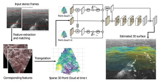
The whole procedure is summarized in Figure 1. WASSfast operates sequentially on the stereo frames according to their acquisition time. In every iteration, it takes as input the stereo pair at time t together with the estimate of the surface spectrum at time $t-1$ (in the first frame, the previous spectrum is assumed to be zero everywhere). Then, the PU approach operates as follows:

• feature detection and optical flow are used to extract a set of matching feature points between left and right images;
• matches are triangulated to obtain a sparse 3D point cloud;
• spectrum at time $\left(t\right)$ (i.e., the current frame) is Predicted from the previous estimate at time $(t-1)$ according to the linear dispersion relation;
• spectrum prediction is updated to fit the triangulated points obtained in step 2. This creates an estimate of the spectrum at time $\left(t\right)$ that is used when processing frames at time $(t+1)$. Thus, the process repeats from step 1.

Considering the obtainable speedup, PU formulation works surprisingly well but contains some intrinsic limitations hindering any further improvement. First, it must process frames sequentially, so no parallel computation can be performed (at least at a frame level). Second, spectrum prediction can only look at the past (previous estimate at time $t-1$) and not the future frames. Using both previous and next frames would probably constrain it better for an improved prediction. Finally, the update step is based on a numerical optimization whose running time depends on the data. Convergence can be quick in some cases (just a few iterations) or very slow in some unlucky circumstances. In practice, the maximum number of iterations can be set by the user, but this will not guarantee the convergence. Thus, on average, the processing speed is 1 Hz, but some frames can take longer than others.

The idea explored in this paper is to substitute steps 3 and 4 with a Convolutional Neural Network trained to directly produce surface grids from the triangulated points. The ill-posedness here is solved by letting the model learn what a physically consistent surface should look like according to what has been seen during the training process. The temporal constraints given by the dispersion relation are embedded in the model by processing 3 frames at once: $(t-1)$, $\left(t\right)$ and $(t+1)$ to produce the surface at time $\left(t\right)$. When operating on the whole sequence, each frame is partially processed three times (as previous, next and current frame) but, apart from that, model execution can be parallelized on the whole sequence. We call this new mode of operation WASSfast CNN.

2.2. Network Architecture

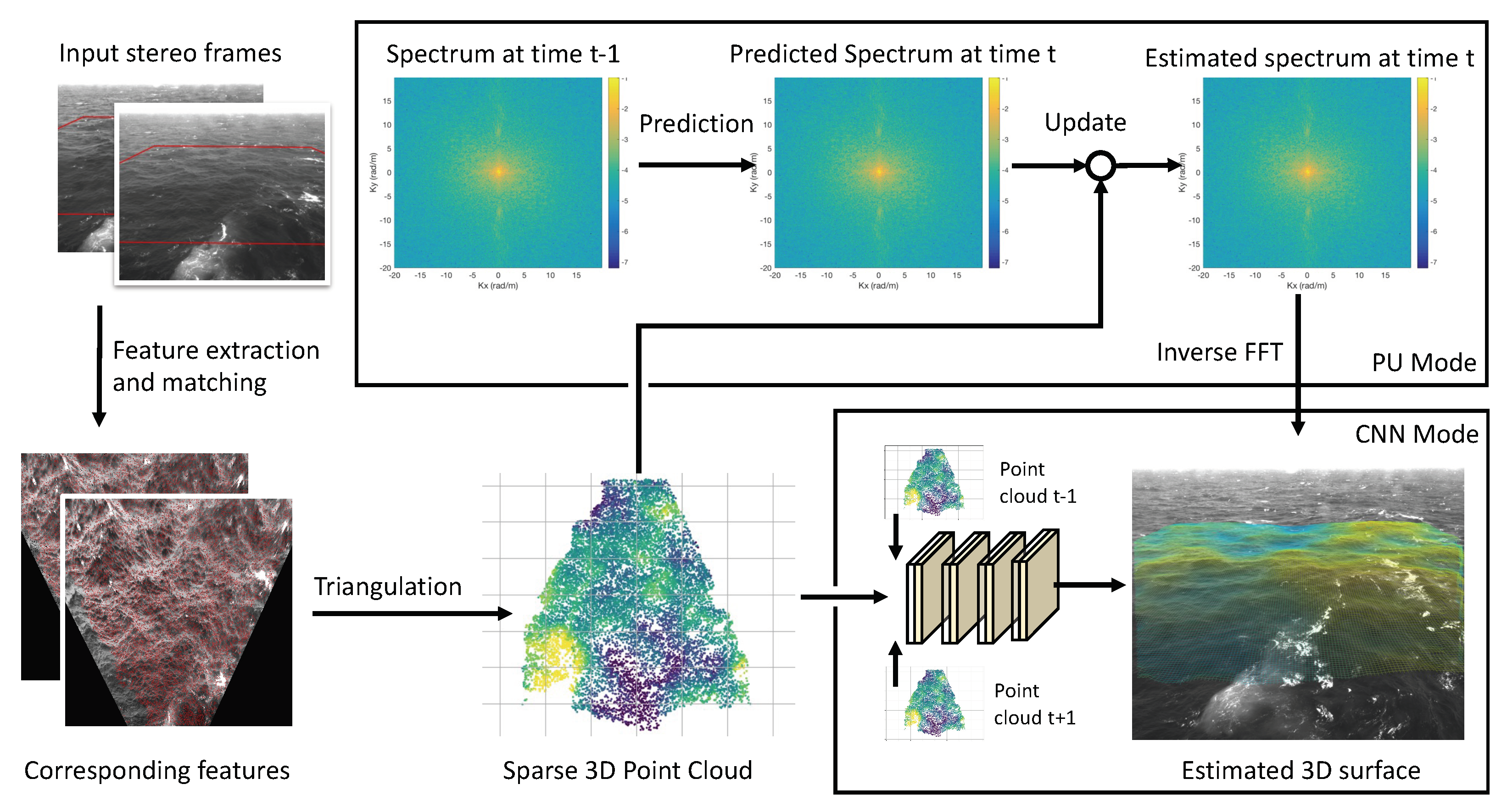
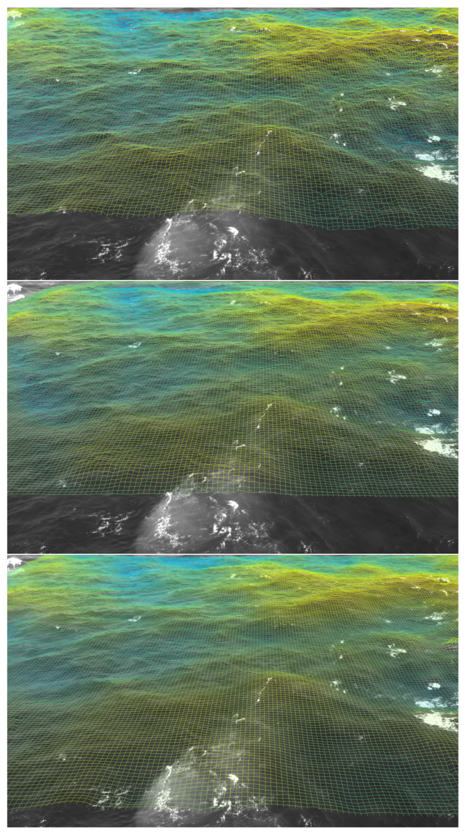
Differently from the PU approach, all the triangulated 3D points are discretized to the defined surface grid before any other operation (Figure 2). This is performed by transforming the point cloud in the mean sea plane reference frame (aligned with the grid), and then projecting each point onto the closest grid node. This operation is implemented simply by discarding the z-coordinate, and rounding the remaining two to the closest integer. This way, the projection is very fast but less accurate compared to the PU approach for two reasons. First, more than one point can end up into the same grid cell. In this case, we just randomly select one of those and discard the others. Second, some information is lost during the discretization since the original “sub-pixel” coordinates are rounded to the closest grid node. This can lead to a cutoff in the high frequencies of the wave spectrum, unless the grid resolution is reasonably high. Nevertheless, this operation is extremely fast, since it can be parallelized with respect to the point cloud, and automatically solves the problem of having two or more points too close together, a critical condition for the convergence of the PU approach.

After point discretization, the problem is simplified from a general 3D surface interpolation to an image processing-based depth completion performed directly on the surface grid. Indeed, our grid can be seen as a 1-channel floating-point image in which each pixel (i.e., cell) denotes either the elevation of the chosen point with respect to the sea plane or a NaN to indicate that no point was discretized into that grid cell. At this point, the task is to “fill” the missing pixels with reasonable values according to the optimal surface we aim to estimate.

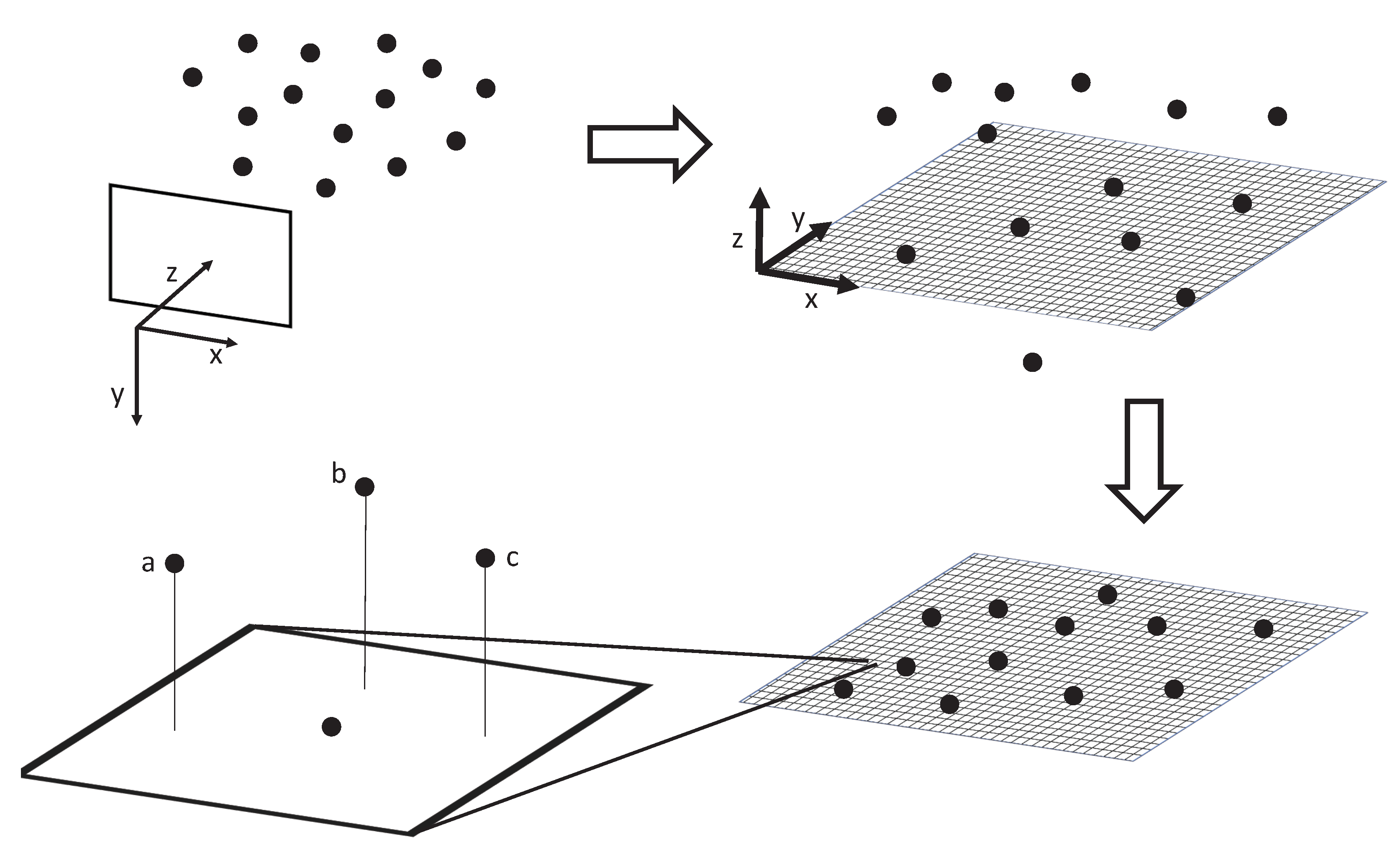
The complete network architecture is displayed in Figure 3. It takes as input three subsequent frames: ${\mathcal{I}}_{t-1},{\mathcal{I}}_t,{\mathcal{I}}_{t+1}$, and produces in output the resulting surface ${\mathcal{O}}_t$ where the missing values have been filled. It is composed by three macro blocks that are executed one after the other. The Depth Completion block implements a preliminary fill of ${\mathcal{I}}_{t-1}$ and ${\mathcal{I}}_{t+1}$ using two instances (with shared weights) of the Depth Completion CNN proposed in [38]. Then, the Temporal Combiner “transports” the sparse points from $t+1$ and $t-1$ onto t to produce an intermediate sparse image $\widehat{\mathcal{I}}$ which is denser than ${\mathcal{I}}_t$. From here, the final Surface Reconstruction part estimates the missing values combining a sequence of Sparse Convolutions with the classical Shepard interpolation [43] (also known as Inverse Distance Weighting, or IDW).

The novelty of our approach, compared to just using a general purpose Depth Completion CNN, is twofold. First, we introduce physical constraints our reconstructed surfaces (in this case, the dispersion relation) since we know that points are samples triangulated from a real sea-surface. Second, we train the network to reconstruct the difference (i.e., the high-frequencies) with respect to a surface already interpolated with a general-purpose method. Experimentally, we observed that this leads to better results than directly reconstructing the final surface (see Section 2.5). In the following sections, we describe each block in detail.

2.3. Depth Completion Block

The depth completion block consists of an end-to-end CNN taking a $256\times 256\times 2$ input tensor and producing a $256\times 256\times 1$ output tensor $\mathcal{S}$. The two input channels are organized as follows: the first channel $\mathcal{I}$ is a floating point image containing some pixels with valid depth values (representing sea-surface elevation at that grid point, normalized in range $0\dots 1$ according to the minimum and maximum value of the batch) and some others corresponding to missing data, arbitrarily filled with zeros. The second channel $\mathcal{M}$ consists of a data mask, i.e., a binary image containing 1 or 0, denoting respectively that the pixel at that coordinate is valid (i.e., the first channel contains an observed value) or not.

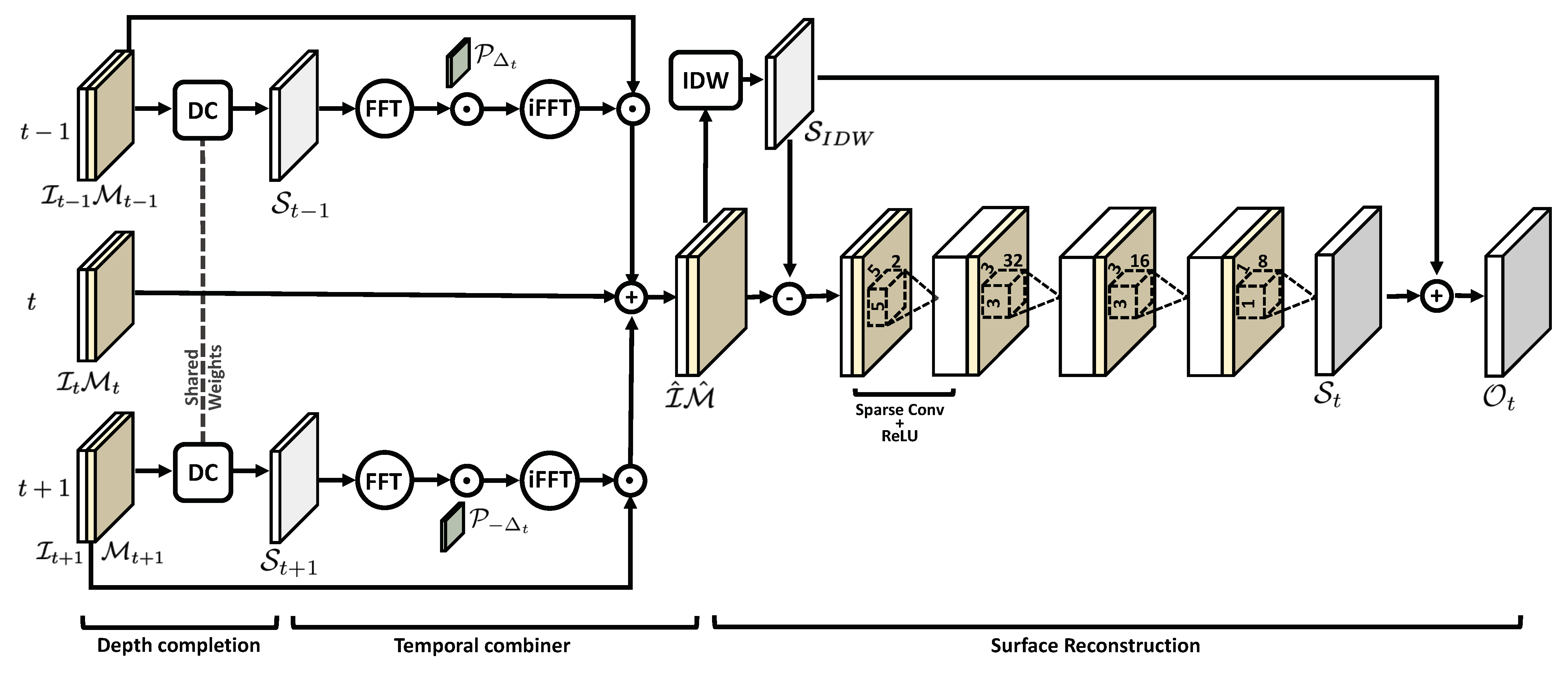
The architecture is a classical feed-forward network as shown in Figure 4: it contains a sequence of five sparse convolution layers, followed by Rectified Linear Unit (ReLU) activations. Each sparse convolution produces a 16-channels output tensor obtained by convolving the input with 16 different trainable kernels with predefined sizes. At the end, a sparse convolution with a single $1\times 1\times 16$ kernel followed by a linear activation produces the resulting dense output surface $\mathcal{S}$.

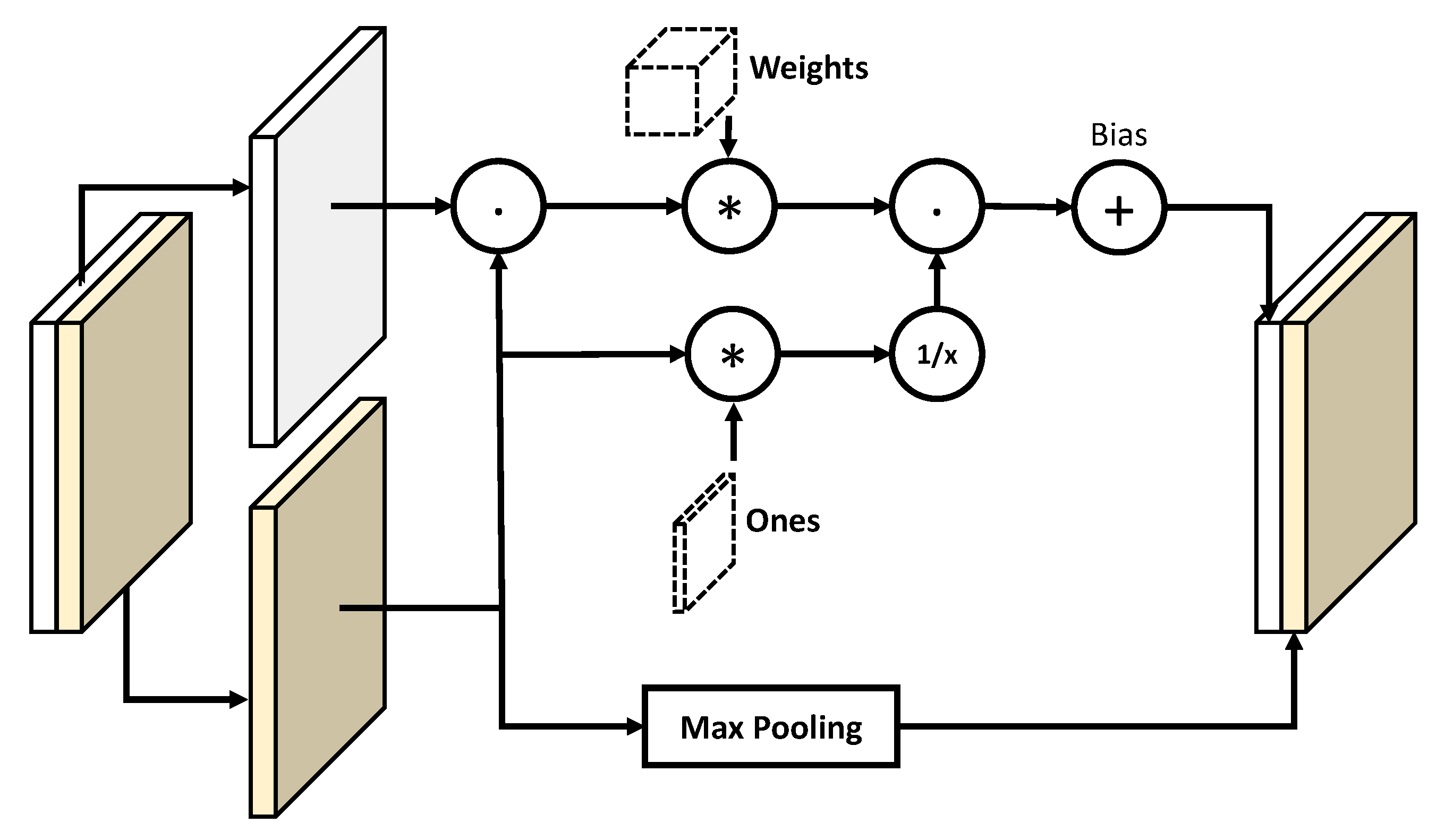
The idea behind sparse convolution is simple but effective in practice. Let the input be a $N\times M\times k$ tensor, composed by the concatenation of a $N\times M\times (k-1)$ tensor representing image data and an $N\times M\times 1$ tensor representing the binary mask (respectively white and yellow blocks in Figure 5). The first data block is multiplied element-wise to the mask to explicitly fill invalid values with zeros (note that valid values remain untouched since they are multiplied by 1). The zero-filled data are convolved as usual, but the result is normalized according to the number of valid values inside the region spanned by the convolution filter. In other words, the normalization factor results in being the number of ones found in the mask within the corresponding convolution window: such factor is simply computed by convolving the mask with a constant kernel composed by all ones, with the same size as the kernel used for data convolution. Finally, the layer output is computed by dividing the convolved data with the convolved mask, and then adding a trainable bias.

At the same time, the mask needs to be updated coherently with the new data in order to propagate the information. This is done by dilating the 1-regions of the mask, performing a max-pooling operation with unitary stride and size equal to the convolution kernel (note that this is equivalent to compute a morphological dilation on the mask). In this way, the valid data values are propagated through the new mask. Assuming to employ v filters for data convolution, the new data and mask are concatenated together to produce the $N\times M\times (v+1)$ output tensor. The whole operation is summarized in Figure 5.

Note that, albeit generic, this block would be sufficient to fill the missing grid values. However, as shown in the experimental section, what follows embeds physical priors to the network and greatly improves the final surface.

2.4. Temporal Combiner Block

The temporal combiner block lies at the core of the proposed WASSfast network: indeed, it is designed to fuse the information coming from three subsequent frames and improve the quality of the final output. The rationale is that each input frame ${\mathcal{I}}_t$ can be seen as a random sampling of the unknown sea surface at time t. Therefore, considering two distinct frames ${\mathcal{I}}_{t_i}$ and ${\mathcal{I}}_{t_j}$, they will contain valid values at different locations. If we imagine to “transport” the valid points from $t_i$ to $t_j$ (or vice-versa), we can increase the sampling density of one of the two images and therefore improve the quality of the final output. This operation is not trivial unless we are able to accurately track the reconstructed points along the frame sequence. Nevertheless, physical priors on the wave dynamics can be taken into account to predict the sea surface at a certain (sufficiently small) time delta ${\Delta }_t$. This is exactly the operation performed by the PU approach during the prediction phase (see [15], Section 2.3 for details). To summarize, it is sufficient to take the 2D Fourier spectrum of the surface at time t, rotate its phases by an angle defined by the linear dispersion relation, and then compute the inverse Fourier transform to obtain the predicted surface at time $t+{\Delta }_t$.

The structure of the temporal combiner is shown in the central part of Figure 3: it takes as inputs the previous ${\mathcal{I}}_{t-1}$, next ${\mathcal{I}}_{t+1}$ and current frame ${\mathcal{I}}_t$ in the sequence being analyzed, together with their associated masks ${\mathcal{M}}_{t-1}$, ${\mathcal{M}}_{t+1}$ and ${\mathcal{M}}_t$.

The depth completion block described in Section 2.3 is applied in parallel (sharing the weights) only on ${\mathcal{I}}_{t-1}$ and ${\mathcal{I}}_{t+1}$. In this way, we obtain the two dense surfaces ${\mathcal{S}}_{t-1}$ and ${\mathcal{S}}_{t+1}$ associated with the previous and next frames, respectively.

At this point, we can exploit the temporal relation between subsequent frames and predict two new surfaces by rotating the phases of ${\mathcal{S}}_{t-1}$ and ${\mathcal{S}}_{t+1}$, assuming a time delta of ${\Delta }_t$ and $-{\Delta }_t$, respectively. This is implemented as an element-wise multiplication between the complex matrix resulting after the 2D Fourier transform of the surface and a phase rotation matrix:

$$\begin{array}{ccc}\hfill {\mathcal{S}}_{t-1}^{\prime }& =& {\mathcal{F}}^{-1}\left(\mathcal{F}\left({\mathcal{S}}_{t-1}\right)\odot {\mathcal{P}}_{{\Delta }_t}\right)\hfill \\ \hfill {\mathcal{S}}_{t+1}^{\prime }& =& {\mathcal{F}}^{-1}\left(\mathcal{F}\left({\mathcal{S}}_{t+1}\right)\odot {\mathcal{P}}_{-{\Delta }_t}\right).\hfill \end{array}$$

(1)

where $\mathcal{F}(·)$ denotes the 2D Fourier transform and ⊙ is the element-wise matrix multiplication. The 2D phase rotation matrix ${\mathcal{P}}_{{\Delta }_t}$ is computed as follows:

$$\begin{array}{ccc}\hfill {\mathcal{P}}_{{\Delta }_t}& =& \left(\begin{array}{c}{A}_{k_x,k_y}\end{array}\right)\hfill \\ \hfill A_{k_x,k_y}& =& e^{i{\Delta }_t{\omega }_{k_x,k_y}}\hfill \\ \hfill {\omega }_{k_x,k_y}& =& sign(s_x{k}_x+s_y{k}_y)g\sqrt{k_x^2+k_y^2}\hfill \end{array}$$

(2)

where $k_x$$k_y$ are the grid wavenumbers, and $s_x,s_y$ are two signs related the main wave propagation direction (The predict step implemented in WASSfast is able to automatically estimate $s_x,s_y$ by analyzing the optical flow between the first two frames).

In this way, ${\mathcal{S}}_{t-1}^{\prime }$ and ${\mathcal{S}}_{t+1}^{\prime }$ are the predicted surfaces at time t computed respectively from ${\mathcal{S}}_{t-1}$ and ${\mathcal{S}}_{t+1}$. In other words, this operation allowed for “moving” both the surfaces to time t, enabling us to merge the resulting data with different random samplings. Then, ${\mathcal{S}}_{t-1}^{\prime }$ and ${\mathcal{S}}_{t+1}^{\prime }$ are sparsified again by filling with zeros all the pixels corresponding to zeros in the original binary masks:

$$\begin{array}{ccc}\hfill {\mathcal{I}}_{t-1}^{\prime }& =& {\mathcal{S}}_{t-1}^{\prime }\odot {\mathcal{M}}_{t-1}\hfill \\ \hfill {\mathcal{I}}_{t+1}^{\prime }& =& {\mathcal{S}}_{t+1}^{\prime }\odot {\mathcal{M}}_{t+1}.\hfill \end{array}$$

(3)

The final step of the temporal combiner consists of blending the obtained values and the current input sparse data ${\mathcal{I}}_t$. First, the three sparse images need to be combined according to possible overlapping. Indeed, since we want to merge in the same image sparse points coming from different random samplings, we need to take care of the pixels for which we have more than one value. For this reason, given a pixel location p, the corresponding values will be weighted as follows:

$$\begin{array}{c}\hfill \widehat{\mathcal{I}}\left(p\right)=\frac{\frac{1-\alpha }{2}{\mathcal{I}}_{t-1}^{\prime }\left(p\right){\mathcal{M}}_{t-1}\left(p\right)+\alpha {\mathcal{I}}_t\left(p\right){\mathcal{M}}_t\left(p\right)+\frac{1-\alpha }{2}{\mathcal{I}}_{t+1}^{\prime }\left(p\right){\mathcal{M}}_{t+1}\left(p\right)}{\frac{1-\alpha }{2}{\mathcal{M}}_{t-1}\left(p\right)+\alpha {\mathcal{M}}_t\left(p\right)+\frac{1-\alpha }{2}{\mathcal{M}}_{t+1}\left(p\right)}\end{array}$$

(4)

where $\alpha \in [0,1]$ is a weighting parameter. In this way, if only one out of three elevation values is present at pixel p, it will be included in the merged image. On the other hand, if we have more than one possible value in p, the final elevation is computed as a weighted sum of the available values. In our tests, we gave a higher relevance to the central frame (i.e., the input data for which we did not apply prediction) by setting $\alpha =0.8$. Note that, with this formulation data in ${\mathcal{I}}_{t-1}^{\prime }$ and ${\mathcal{I}}_{t+1}^{\prime }$ being weighted equally, there could be some cases for which they should be treated differently, for example if the frame rate is not constant. Indeed, the adaptation of such weighting parameters could be further investigated in some future work. After the operation described in Equation (4), the sparse image $\widehat{\mathcal{I}}$ incorporates sparse points coming from the three input frames, exploiting the prediction step. The associated mask is simply computed as the element-wise logical or among the three input masks:

$$\widehat{\mathcal{M}}={\mathcal{M}}_{t-1}\vee {\mathcal{M}}_t\vee {\mathcal{M}}_{t+1}.$$

(5)

Given the different random sampling at each frame, this new sparse image $\widehat{\mathcal{I}}$ will be denser with respect to the three inputs taken separately, with the advantage of possibly improving the final surface quality and constraining the temporal evolution of the surfaces according to the data acquired immediately before and after the currently reconstructed frame. Note two interesting features of the temporal combiner. First, the Fourier Transform and point blending are all linear operations that can be easily differentiated so it does not pose any problem for the back-propagation [44] (Chapter 6.5). Second, the temporal combiner does not contain any weight to be trained. After this part, the pair $(\widehat{\mathcal{I}},\widehat{\mathcal{M}})$ is then used as an input for the reconstruction block.

2.5. Surface Reconstruction Block

The surface reconstruction block is added after the temporal combiner, taking as input the sparse data $\widehat{\mathcal{I}}$ and the mask $\widehat{\mathcal{M}}$. At this stage, $\widehat{\mathcal{I}}$ is denser than the original ${\mathcal{I}}_t$, but tends to exhibit regions where no samples at all are present. These “holes” in the data typically occur on the back-side (with respect to the camera viewpoint) of high waves or in areas where no photometrically distinctive features are present (like in flat white-capped regions formed by breaking waves).

We observed that just using the depth completion block (Figure 4) fails to both preserve details where many samples are present and close the larger holes. The problem is that the sparse convolutions must have a limited extent ($3\times 3$ or $5\times 5$) to be effectively trained, but that means increasing the network depth to accommodate sparser regions. However, in all our tests, we observed that the deeper the network, the smoother the resulting output tends to be. One solution might be to use a multi-scale depth completion network [39] in this last stage, but such architecture is more complex and therefore harder to train and slower during its usage. Thus, we explored a different approach in which sparse convolutions are used only to improve the surface’s small details.

It is easy to note that the classical Shepard interpolation (in its simple form, without taking into account local gradients) is a non-trainable instance of a sparse convolution (see Figure 5). In addition, known as Inverse Distance Weighting, the idea is to fill a missing value with the average of the valid neighboring pixels, weighted by a negative power of their distance. If we restrict the averaging neighborhood to a fixed maximum radius, its implementation can be realized by convolving both the sparse data and mask with a kernel filled with values that are proportional to the distance from the central pixel. After that, the convolved image is divided element-wise with the convolved mask to obtain a dense surface. Since the IDW kernel values are not trainable, its impact on our model is negligible even when using window sizes several time bigger than the ones used for sparse convolutions. Thus, we decided to mix the two approaches to take the best of the two worlds.

The idea is to create a coarse surface using IDW, and then “add” the additional details with the usual depth completion network that learns to refine the final surface. Indeed, the obtained surface ${\mathcal{S}}_{IDW}$ is initially subtracted from the sparse points $\widehat{\mathcal{I}}$ (essentially like in a high-pass filter), then a series of four sparse convolutions with ReLU activations are performed on sparse data. Finally, the surface ${\mathcal{S}}_{IDW}$ is added back to $\widehat{\mathcal{I}}$ to obtain the final output surface.

3. Network Training

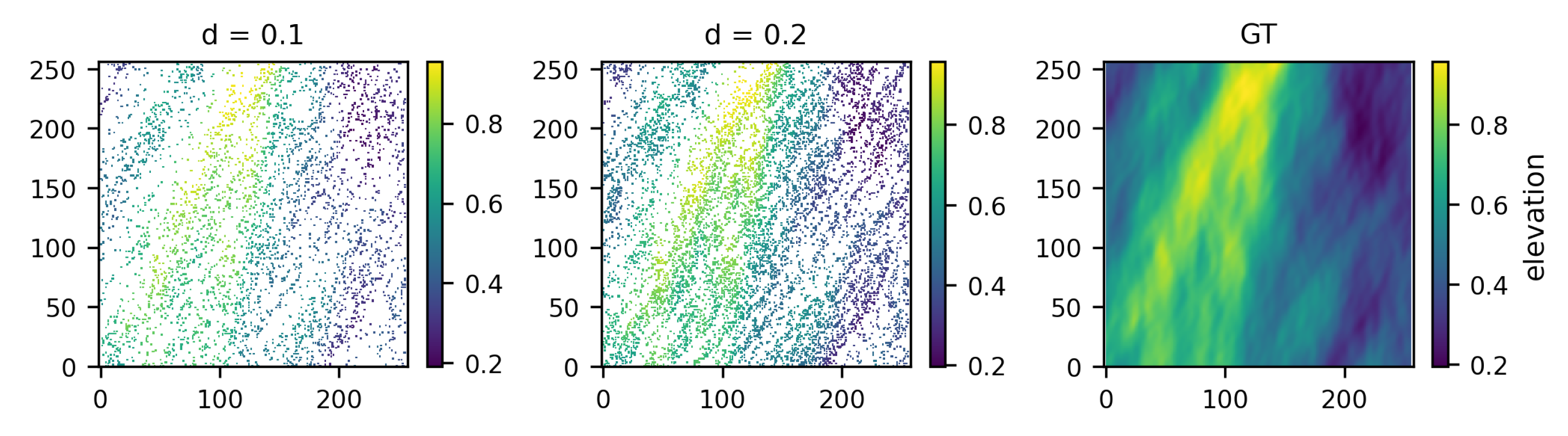
To be properly trained, WASSfast CNN requires several input–output samples, like the ones shown in Figure 6. One possibility is to use WASS as a reference surface reconstruction method to generate the expected output surfaces. We discarded this alternative for the following reasons:

• Training data should be as heterogeneous as possible to comprise different wave direction, sampling density, frame rates, etc. This requires great effort in organizing a vast set of WASS processed data that would be impractical. Moreover, in this way, we are not ensured to capture as many conditions as possible to avoid overfitting.
• WASS data partially suffers from depth quantization produced by the dense stereo approach. If used for training data without proper filtering, the CNN would probably learn to “simulate" the quantization effect along the image scanlines;
• A vast amount of data needed to train a Deep Neural Network model without overfitting. We currently do not have enough data to ensure proper training, and data augmentation is a partially viable option since it is difficult to define image transformations to realistically simulate different view angles, wave directions, lighting conditions, etc.

To overcome these problems, we used the Matlab package WAFO [45] to generate training and test data in a completely synthetic way. Specifically, we generated several scenarios comprising linear and nonlinear Gaussian waves in an area with a similar extent of the one used in previous WASS setups (see

Table 1. Parameters used to generate different scenarios used for training.

Parameter	Value
Grid size	$256\times 256$
Grid cell size (m)	$0.46$
Frame rate (Hz)	7
Significant wave height Hm0 (m)	Random uniform in range $[5.0\dots 8.0]$
Primary peak period Tp (s)	Random uniform in range $[7.2\dots 8.8]$
Spreading parameter Sp (deg)	Random uniform in range $[15.0\dots 22.0]$
Wave direction ${\theta }_0$ (rad)	Random uniform in range $[0\dots 2\pi ]$
Number of frames	700

for details).

Each scenario is composed by a sequence of sea surfaces ${\overline{\mathcal{O}}}_t$ sampled on a regular $256\times 256$ grid at a frame rate of 7 Hz, simulated using the bimodal (swell+wind) Torsethaugen spectral density model implemented in WAFO. Sea-state parameters are randomized to simulate a wide range of conditions that can be considered reasonable for a typical WASSfast installation on an offshore research platform. All the generated surfaces are the expected outputs of our CNN, divided into training and testing sets. In detail, for training data, we generated 200 different scenarios: for each one, we selected 64 frames, for a total of 12,800 different surfaces (each one with corresponding previous and next frames). The test set includes 100 scenarios, each one including 32 frames, for a total of 3200 surfaces.

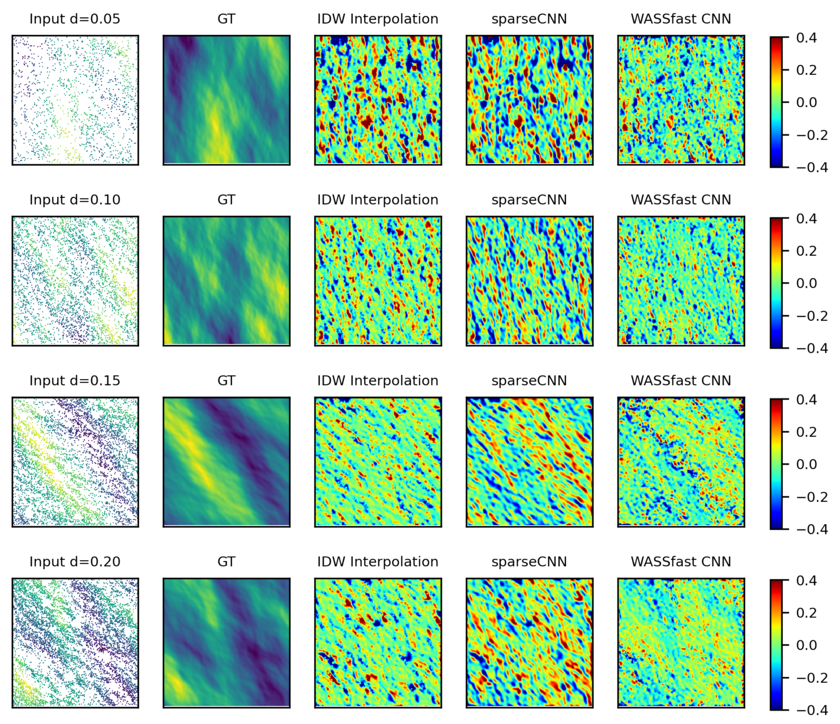
To generate the sparse input ${\mathcal{I}}_t$ we designed a specific sampling procedure so that the resulting points exhibit features as close as possible to an actual stereo acquisition.

We opted for a non-uniform sampling of each surface ${\overline{\mathcal{O}}}_t$: we did this by associating each grid point $(x,y)$ with a different probability of being observed: we denote such probability as $p_{{\overline{\mathcal{O}}}_t}(x,y)$. All points have the same “initial” probability of being sampled, equal to $d\in [0,1]$. In this way, we ideally obtain a uniform sampling with density d: we will address to such variable d in the rest of the paper as the density parameter for data generation. Then, we simulated waves self-occlusion by decreasing with a factor $q\in [0,1]$ the probability for a point to be observed only if it exhibits a negative gradient on the y-direction (In our experiments, we kept a fixed $q=0.2$). Therefore, given a surface ${\overline{\mathcal{O}}}_t$, we define $p_{{\overline{\mathcal{O}}}_t}(x,y)$ as follows:

$$p_{{\overline{\mathcal{O}}}_t}(x,y)=\left\{\begin{array}{cc}dq\hfill & \mathrm{if}\frac{\partial {\overline{\mathcal{O}}}_t}{\partial y}(x,y)<0\hfill \\ d\hfill & \mathrm{otherwise}.\hfill \end{array}\right.$$

(6)

The input image ${\mathcal{I}}_t$ is then computed sampling surface ${\overline{\mathcal{O}}}_t$ according to the outcome of a random variable $X_{{\overline{\mathcal{O}}}_t}$ following a Bernoulli distribution:

$$\begin{array}{c}\hfill X_{{\overline{\mathcal{O}}}_t}(x,y)\sim Ber\left(p_{{\overline{\mathcal{O}}}_t}(x,y)\right)\\ \hfill {\mathcal{I}}_t(x,y)={\overline{\mathcal{O}}}_t(x,y)X_{{\overline{\mathcal{O}}}_t}(x,y).\end{array}$$

(7)

In this way, we obtain a non-uniform sampling that is coherent with the waves direction and the (virtual) stereo cameras capturing the scene.

Figure 6 displays the resulting points applying respectively a low sampling ratio ($d=0.1$, left) and a higher one ($d=0.2$, center), together with the Ground Truth surface (GT). Moreover, we introduced random holes, i.e., areas where surface points are completely missing. This aspect is also fundamental for simulating real-world data since the acquired point clouds may exhibit missing data in relatively large areas. To this end, we introduced a parameter $ma{x}_h$ representing the maximum number of holes appearing in a single frame: each image will therefore include a random number of holes in the interval $[0,\cdots ,ma{x}_h]$. Each generated hole is also characterized by a variable size, uniformly selected in the range $[mi{n}_r,ma{x}_r]$ and by a variable shape, expressed as a covariance value in the range $[mi{n}_{cov},ma{x}_{cov}]$.

3.1. Loss Function

As mentioned before, the training process aims at estimating the weights of the neural network model (i.e., the values of convolution kernels and biases) so that the produced output ${\mathcal{O}}_t$ is as similar as possible to the true output ${\overline{\mathcal{O}}}_t$. This notion of similarity is given by the so-called Loss Function that gives a penalty factor depending on how much ${\mathcal{O}}_t$ is different from the correct output.

Needless to say that the loss function plays a crucial role to let the network behave as expected. A sophisticated loss function may better account for challenging situations at a price of a more unstable gradient during training phase with the consequent risk of being stuck on a local minima. Several loss functions have been proposed in the literature when working with Neural Networks for image processing [46]. In the case of our application, we used a combination of L1 loss and Structural Similarity Index (SSIM) proposed by Wang et al. [47] weighted by a factor $\lambda$ (set to $0.84$ in all our experiments). The complete loss function used for training is shown in Equation (8):

$$\mathcal{L}({\overline{\mathcal{O}}}_t,{\mathcal{O}}_t)=(1-\lambda )|{\overline{\mathcal{O}}}_t-{\mathcal{O}}_t|+\lambda SSIM({\overline{\mathcal{O}}}_t,{\mathcal{O}}_t)$$

(8)

3.2. Training Process

As previously discussed, the proposed WASSfast CNN is composed by three main blocks: depth completion, temporal combiner, and surface reconstruction. The depth completion task plays a fundamental role for the surface reconstruction, since its output is directly used in the prediction step of the temporal combiner to merge frames at different times and obtain a denser set of points. Needless to say, the temporal combiner presented in our architecture is effective only if the depth completion block produces a reasonable estimate of the correct underlying surface. When the training process is started, this unlikely happens since the initial weights are randomly generated. Therefore, at an initial training stage, the temporal combiner will “scramble" the phases of completely random surfaces, producing outputs significantly far from the actual surface. This makes the whole optimization highly unstable and hard to converge in practice.

Note that the trainable parts of the network are the initial depth completion block (repeated for input at times $t-1$ and $t+1$) and the weights of sparse convolutions involved in the final reconstruction step. Indeed, the depth completion block can be seen as an independent sub-network, producing a dense surface from sparse input points. For this reason, we decided to first train the depth completion block as a standalone network: in this way, we can plug the (very close to optimal) weights in the complete WASSfast CNN network and proceed with global optimization avoiding training instability. Hence, the training process is divided into two steps:

• The depth completion block alone (Figure 4) is trained on the whole dataset until convergence.
• The full WASSfast CNN (with temporal combiner and surface reconstruction) is trained introducing the depth completion block weights already trained in the first step.

In this way, the depth completion block is optimized beforehand so its initial weights (when the full network train is performed) are already close to the global optimum.

Moreover, while training the depth completion block, we observed that changes in the density of training data have a significant effect on the reconstruction accuracy. We experimentally observed that starting with a relatively high sample density and gradually lowering its value throughout the optimization leads to a quicker and more stable convergence. The concept of presenting to the network gradually complex examples during training is addressed in the literature as curriculum learning [48,49,50]. In some cases, such a method is shown to be an effective training strategy, leading to fast and stable convergence and to a better network generalization.

We train the depth completion block in groups of several epochs, reducing the sample density range in each group and testing the resulting loss on a separated validation set, according to the following schedule:

• 50 epochs, sampling $d\sim U(0.15,0.20)$
• 50 epochs, sampling $d\sim U(0.10,0.15)$
• 70 epochs, sampling $d\sim U(0.05,0.10)$
• 70 epochs, sampling $d\sim U(0.03,0.05)$

where $U(a,b)$ denotes a uniform distribution over the interval $[a,b]$. After that, we filled the pre-trained weights in the depth completion block and trained the full network for 50 more epochs, until the loss shows no significant change between each iteration. For this last step, we restrict the input density d in $[0.10,0.2]$, since it represents closely the density of real-world data. For the IDW convolution part, we empirically identified a good kernel, namely a $21\times 21$ matrix with its values set equal to the distance from the window center to the power of $-2.8$. Considering the density of our data, we found this configuration of IDW to be suitable to obtain a smooth initial surface without introducing artifacts.

In both of the training steps, we employed all the surfaces generated in the training set and randomly generated sparse input data with holes as described previously, with $ma{x}_h=5$ and $mi{n}_r=20,ma{x}_r=50$ (in pixels). Note that the random generation of the input points takes place at the beginning of each epoch, so the network is constantly feed with new patterns of sparse data, avoiding overfitting. In all cases, we used the the Adam optimizer with an adaptive learning rate, starting from ${10}^{-3}$ and automatically decreased to a minimum of ${10}^{-5}$ according to the slope of the loss function during the training.

4. Experimental Results

In order to analyze the quality of the sea surface reconstruction using our approach, we divided the experimental validation into two parts. First, we tested the depth-completion capability of the proposed WASSfast CNN against another CNN-based method and a non-learning interpolation approach. Since this kind of comparison requires the availability of an accurate ground truth, we performed such experiments exploiting only the synthetically generated data (the test set as described in Section 3). After that, we tested the proposed WASSfast CNN system by embedding the CNN-based surface reconstruction technique directly in the reconstruction pipeline with real-world data. In this way, we were also able to compare the results obtained with the CNN-based approach against WASSfast PU and WASS.

4.1. Comparison against Synthetic Data

To compare our method with other depth completion techniques, we employed the synthetic sea surfaces in the test set created as shown in Table 1. We compared WASSfast CNN with the sparsity-invariant CNN performing depth completion proposed in [38] (denoted as SparseCNN). Moreover, we applied a non-learning algorithm for depth completion, consisting of a simple IDW operation with a fixed kernel. The rationale of this comparison is to test the actual ability of the proposed architecture to blend three frames and generate a more accurate surface with respect to other methods employing only the input sparse data.

Figure 7 (first row) shows the Mean Absolute Error (MAE) and Peak Signal to Noise Ratio (PSNR) for our method, SparseCNN, and IDW varying the density of input data from $d=0.05$ to $d=0.20$. Error bars show the standard deviation obtained running the methods on all of the different scenarios included in the test data. We can observe that the proposed architecture outperforms both techniques, exhibiting a better accuracy in all the cases. As expected, the overall reconstruction quality increases proportionally with the point density. Surprisingly, IDW works better than SparseCNN, especially the point density increases. This validates the fact that SparseCNN tends to overfit to the amount of points it has seen during the training. Therefore, to ensure a good quality for sparse regions, it over-smooths areas where finer details are present. On the other hand, our network exploits successfully the temporal relation between the frame to be reconstructed and its previous and next, effectively improving the surface accuracy on finer details. In Figure 7 (second row), we show the effect of interpolation on the frequency spectra. To evaluate that, we generated two 10 min long synthetic sequences, with sampling $d=0.08$ and $d=0.2$, respectively, and extracted a timeseries at the center of the reconstruction grid. Then, we used the WAFO’s dat2spec function to estimate the one-sided spectral density from data. We can observe how the spectrum obtained with WASSfast CNN (blue line) is more similar to the Ground Truth (black line) especially at frequencies ranging from $0.25$ to $0.38$ rad/m where other methods undershoot the energy contribution. There is a plateau starting at $0.58$ rad/m, where the spectra of all the methods are not reliable anymore. At low frequencies, below $0.04$ rad/m, our approach also performs better than IDW and SparseCNN, but the difference is less noticeable.

Figure 8 and Figure 9 display some qualitative results from different samplings and scenarios. In all cases, surfaces produced by WASSfast CNN are qualitatively better with respect to other methods. Indeed, the full WASSfast network output exhibits more details, especially at high frequencies, where they are difficult to recover due to a particularly sparse sampling. Moreover, the predicted output shows no spikes or artifacts regardless of the sampling position of the input points. Instead, PU mode may fail to converge whenever two input points are spatially close, as reported in the original paper.

4.2. Comparison on Real Data

Experiments on real data were performed using three records acquired in 2018 at the Gageocho ORS managed by the Korea Institute of Ocean Science and Technology (KIOST). We used the same dataset described in [3,15] for a direct comparison between the well known WASS pipeline [12], WASSfast working with the existing PU mode, and the newest developed CNN mode.

Such data were recorded after the passage of the tropical storm Kong-rei, originated from a tropical disturbance in the open Pacific Ocean. For a couple of days, it went westward, organizing into a tropical depression on 27 September. Then, it intensified into a powerful Category 5 super-typhoon early on 2 October. The data used in our study were recorded on 6 October when Kong-rey made landfall in Tongyeong (South Gyeongsang Province in South Korea) as a high-end tropical storm, transitioned a few hours later into an extratropical cyclone, while impacting southern Hokkaido, such as areas near Hakodate. Sequences are composed by 2000 stereo frames acquired at a frame rate of $7.5$ Hz, distributed along the day at 10:00 a.m., 2:00 p.m. and 5:00 p.m. local time (see

Table 2. The three stereo sequences used to compare the two WASSfast reconstruction modes against the old WASS pipeline.

Record Name	Time	Location	Rate	Length
G201810061000	6 October 2018, 10:00 UTC9	Gageocho ORS	$7.5$ Hz	2000 frames
G201810061400	6 October 2018, 14:00 UTC9	Gageocho ORS	$7.5$ Hz	2000 frames
G201810061700	6 October 2018, 17:00 UTC9	Gageocho ORS	$7.5$ Hz	2000 frames

for details).

For the processing, we used a consumer high-end desktop PC equipped with an Intel Core i9-9900K CPU running at a 3.6 Ghz (peak) and a single Nvidia GeForce RTX 2080 with the software compiled and running natively on Windows 10. We started by reconstructing the three sequences with WASS to obtain the corresponding dense point clouds. Then, the mean sea plane was estimated to define the square grid surface measuring $128\times 128$ m divided into $256\times 256$ nodes (grid resolution 0.5 m). Area spans starting from ≈36 m away from the camera up to 163 m in the farthest point. As common in the literature, WASS’ surface used for reference was gridded from each point cloud using the Matlab scatteredinterpolant function. It works by computing a Delaunay’s triangulation of the data points to linearly interpolate grid points inside each triangle. Average running time was ≈0.7 frames per second (FPS) for WASSfast PU and ≈5 FPS WASSfast CNN. Standard WASS gridding took more than a minute per frame.

4.2.1. Time Series Comparison

In Figure 10, we compare the surface elevation time series extracted at the grid center, corresponding to the x–y coordinates $(-0.35,-70.35)$ m with respect to the right camera reference frame (Figure 11 bottom-right). The time series produced by WASSfast (both modes) are very similar to the ones produced by WASS. However, as observed in [15], WASSfast tends to produce a smoother surface elevation field since the total number of triangulated points are a fraction of the ones produced by WASS resulting in a lower spatial resolution.

The output of WASSfast while running in CNN mode is very similar to the one produced in PU mode. This is evident for sequence G201810061000 and G201810061700, characterized by better contrast and exhibiting a higher number of triangulated points. The Pearson’s coefficient between WASS and WASSfast CNN is on the order of $0.98$, with the CNN mode performing better than PU for the two aforementioned sequences (exact coefficients reported in Figure 10). Only in sequence G201810061400 did the CNN mode performed slightly worse, even if the difference is almost negligible.

Overall, the two modes appear to be really similar when comparing time series extracted at the center of the grid, showing that the proposed Deep Neural Network was effectively trained to accurately reconstruct sea surfaces from sparse scattered data. Considering the speedup obtained for the processing, this novel mode is certainly promising for future extensive application.

4.2.2. Sea-Waves Spectrum

After assessing that WASSfast CNN is able to produce surface elevations close to the ones produced by WASS, we analyzed the space-time spectra of the three Gageocho sequences to evaluate if it is also possible to reliably characterize the sea-state condition.

We used the spatio-temporal sea surface elevation fields $z(x,y,t)$, computed with the two WASSfast modes, to characterize the spectral and statistical properties of the wave field. We assume it to be statistically homogeneous in its spatial extent and stationary within the time interval of each record. Thus, from each $z(x,y,t)$, the 3D spectrum $S(K_x,K_y,{\omega }_a)$ was obtained using the 3D Discrete Fourier transform and analyzed to compare the energy distribution at different wavenumbers and frequencies. Then, we integrated the 3D spectrum along all the directions to obtain the omni-directional apparent frequency variance density spectrum (Figure 11).

In all three sequences, we observe a good localization of the peak frequency and almost the same energy response from frequencies ranging from $0.01$ to $0.5$ rad/s, in accordance with what was previously observed in the synthetic tests. At lower and higher frequencies, the various approaches slightly diverge. Both PU and CNN modes have a lower energy response at higher frequencies, with CNN lower than PU, showing in general that the surface produced by the CNN tends to be less noisy than the other. It has to be noted, however, that the spectrum update step of WASSfast PU can be tuned to weight the high-frequencies cutoff between the data and the predicted previous surface. This cannot be controlled in CNN mode as it is automatically learned by the network during the training. Interestingly, we observe that the CNN mode works better than PU mode at low frequencies ranging from $0.01$ to $0.1$ rad/s where the latter tend to underestimate the energy involved. Sequence G201810061400 shows a slightly different spectrum than the other two, and that may be the reason why the Pearson’s correlation for that timeseries is slightly worse for the CNN mode.

Additionally, in Figure 12, we compared some sections of the 3D spectrum $S(K_x,K_w,{\omega }_a)$ at $\omega =0.3,0.4,0.5$ Hz for the record G20200916T010003 computed with PU and CNN mode. It is interesting to observe that PU suffers some energy loss at a certain portion of the spectrum, as reported in [15]. Note, for instance, that, at $0.5$ Hz, the top-left section of the spectrum is noisier than the bottom right half. The new CNN approach seems not to be affected by this problem, even if it uses the same principle of PU mode for predicting the wave spectra among different frames. We think that the final surface reconstruction part of the network is able to compensate this energy loss more efficiently than the update step of the WASSfast PU mode. This behavior is very interesting and will be investigated in the near future.

4.2.3. Qualitative Results

For all the processed sequences, we plotted the resulting reconstructed surfaces on top of the original images. The rendering is performed using the freely available wassncplot tool (https://github.com/fbergama/wassncplot, accessed on 20/05/2021, which renders the produced NetCDF space-time elevation fields $z(x,y,t)$ to a wireframe colored grid.

In Figure 13, we show some selected frames from the same Gageocho sequences used for spectra analysis. WASSfast CNN looks slightly smoother than the others but exhibit a less spiky behaviour in problematic areas at the far end of the reconstruction grid. Note also that the WASSfast CNN grid has a full extent of $256\times 256$ with no weighting window involved (as in PU mode where the window is used to avoid spectral leakage when rotating the harmonics). Full length videos are available as Supplemental Material.

5. Conclusions

We studied a new data-driven approach for 3D reconstruction of sea waves. By reusing the sparse feature matcher implemented in WASSfast, we posed the problem as a Depth Completion scenario for which modern Deep Learning approaches have demonstrated to be very effective. Our novel Convolutional Neural Network architecture is based on the Sparse-CNN but takes into account the temporal evolution of the sea surface under study. In particular, we exploit the linear dispersion relation to increase the sampling density and to enforce temporal smoothness among consecutive frames. Moreover, the final surface reconstruction stage learns to reconstruct the high frequency details by estimating the residuals with respect to a non-trainable, but highly efficient, Inverse Distance Weighting based interpolation.

Experiments on both synthetic and real-world data show that the new approach leads to a more accurate reconstruction, especially at high frequencies, while being almost five times faster than other methods. Considering the significant speedup obtained for the processing, this approach is certainly promising for future implementation as a continuous acquisition and monitoring system of directional wave spectra.

Code is available at https://gitlab.com/fibe/wassfast.

References

1. Benetazzo, A.; Barbariol, F.; Bergamasco, F.; Torsello, A.; Carniel, S.; Sclavo, M. Observation of extreme sea waves in a space-time ensemble. J. Phys. Oceanogr. 2015, 45, 2261–2275. [Google Scholar] [CrossRef] [Green Version]
2. Alvise, B.; Barbariol, F.; Bergamasco, F.; Carniel, S.; Sclavo, M. Space-time extreme wind waves: Analysis and prediction of shape and height. Ocean Model. 2017, 113, 201–216. [Google Scholar] [CrossRef]
3. Benetazzo, A.; Barbariol, F.; Bergamasco, F.; Bertotti, L.; Yoo, J.; Shim, J.S.; Cavaleri, L. On the extreme value statistics of spatio-temporal maximum sea waves under cyclone winds. Prog. Oceanogr. 2021, 197. [Google Scholar] [CrossRef]
4. Filipot, J.F.; Guimaraes, P.; Leckler, F.; Hortsmann, J.; Carrasco, R.; Leroy, E.; Fady, N.; Accensi, M.; Prevosto, M.; Duarte, R.; et al. La Jument Lighthouse: A real scale laboratory for the study of giant waves and their loading on marine structures. Philos. Trans. R. Soc. 2019, 377, 20190008. [Google Scholar] [CrossRef] [Green Version]
5. Stringari, C.E.; Prevosto, M.; Filipot, J.F.; Leckler, F.; Guimarães, P.V. A New Probabilistic Wave Breaking Model for Dominant Wind-Sea Waves Based on the Gaussian Field Theory. J. Geophys. Res. Ocean. 2021, 126, e2020JC016943. [Google Scholar] [CrossRef]
6. Douglas, S.; Cornett, A.; Nistor, I. Image-Based Measurement of Wave Interactions with Rubble Mound Breakwaters. J. Mar. Sci. Eng. 2020, 8, 472. [Google Scholar] [CrossRef]
7. Zappa, C.J.; Banner, M.L.; Schultz, H.; Corrada-Emmanuel, A.; Wolff, L.B.; Yalcin, J. Retrieval of short ocean wave slope using polarimetric imaging. Meas. Sci. Technol. 2008, 19, 055503. [Google Scholar] [CrossRef]
8. Young, I.R.; Rosenthal, W.; Ziemer, F. A Three-Dimensional Analysis of Marine Radar Images for the Determination of Ocean Wave Directionality and Surface Currents. J. Geophys. Res. 1985, 90, 1049–1059. [Google Scholar] [CrossRef] [Green Version]
9. Nieto Borge, J.; Reichert, K.; Hessner, K. Detection of spatio-temporal wave grouping properties by using temporal sequences of X-band radar images of the sea surface. Ocean Model. 2013, 61, 21–37. [Google Scholar] [CrossRef]
10. Jähne, B.; Klinke, J.; Waas, S. Imaging of short ocean wind waves: A critical theoretical review. J. Opt. Soc. Amer. A Opt. Image Sci. Vis. 1994, 11, 2197–2209. [Google Scholar] [CrossRef]
11. Benetazzo, A.; Fedele, F.; Gallego, G.; Shih, P.C.; Yezzi, A. Offshore stereo measurements of gravity waves. Coast. Eng. 2012, 64, 127–138. [Google Scholar] [CrossRef] [Green Version]
12. Bergamasco, F.; Torsello, A.; Sclavo, M.; Barbariol, F.; Benetazzo, A. WASS: An open-source pipeline for 3D stereo reconstruction of ocean waves. Comput. Geosci. 2017, 107, 28–36. [Google Scholar] [CrossRef]
13. Gallego, G.; Yezzi, A.; Fedele, F.; Benetazzo, A. Variational stereo imaging of oceanic waves with statistical constraints. IEEE Trans. Image Process. 2013, 22, 4211–4223. [Google Scholar] [CrossRef] [Green Version]
14. Guimarães, P.V.; Ardhuin, F.; Bergamasco, F.; Leckler, F.; Filipot, J.F.; Shim, J.S.; Dulov, V.; Benetazzo, A. A data set of sea surface stereo images to resolve space-time wave fields. Sci. Data 2020, 7, 145. [Google Scholar] [CrossRef] [PubMed]
15. Bergamasco, F.; Benetazzo, A.; Yoo, J.; Torsello, A.; Barbariol, F.; Jeong, J.Y.; Shim, J.S.; Cavaleri, L. Toward real-time optical estimation of ocean waves’ space-time fields. Comput. Geosci. 2021, 147. [Google Scholar] [CrossRef]
16. Bertero, M.; Boccacci, P. Introduction to Inverse Problems in Imaging; CRC Press: Boca Raton, FL, USA, 1998; ISBN 9780750304351. [Google Scholar]
17. Keller, J.B. Inverse Problems. Am. Math. Mon. 1976, 83, 107–118. [Google Scholar] [CrossRef]
18. Shemdin, O.H.; Tran, H.; Wu, S. Directional Measurement of Short Ocean Waves With Stereophotography. J. Geophys. Res. 1988, 93, 13891–13901. [Google Scholar] [CrossRef]
19. Shemdin, H.; Tran, H.M. Measuring short surface waves with stereophotography. Photogram. Eng. Remote Sens. 1992, 93, 311–316. [Google Scholar]
20. Banner, M.L.; Jones, I.S.F.; Trinder, J.C. Wavenumber spectra of short gravity waves. J. Fluid Mech. 1989, 198, 321–344. [Google Scholar] [CrossRef]
21. Scharstein, D.; Szeliski, R. A Taxonomy and Evaluation of Dense Two-Frame Stereo Correspondence Algorithms. Int. J. Comput. Vis. 2002, 47, 7–42. [Google Scholar] [CrossRef]
22. Benetazzo, A. Measurements of short water waves using stereo matched image sequences. Coast. Eng. 2006, 53, 1013–1032. [Google Scholar] [CrossRef]
23. Wanek, J.M.; Wu, C.H. Automated trinocular stereo imaging system for three-dimensional surface wave measurements. Ocean Eng. 2006, 33, 723–747. [Google Scholar] [CrossRef]
24. Gallego, G.; Benetazzo, A.; Yezzi, A.; Fedele, F. Wave Statistics and Spectra via a Variational Wave Acquisition Stereo System. In Proceedings of the ASME 2008 27th International Conference on Offshore Mechanics and Arctic Engineering, Estoril, Portugal, 15–20 June 2008; pp. 801–808. [Google Scholar]
25. Gallego, G.; Yezzi, A.; Fedele, F.; Benetazzo, A. A Variational Stereo Method for the Three-Dimensional Reconstruction of Ocean Waves. Geosci. Remote Sens. IEEE Trans. 2011, 49, 4445–4457. [Google Scholar] [CrossRef]
26. Vieira, M.; Guimarães, P.; Violante-Carvalho, N.; Benetazzo, A.; Bergamasco, F.; Pereira, H. A low-cost stereo video system for measuring directional wind waves. J. Mar. Sci. Eng. 2020, 8, 831. [Google Scholar] [CrossRef]
27. Benetazzo, A.; Bergamasco, F.; Yoo, J.; Cavaleri, L.; Kim, S.S.; Bertotti, L.; Barbariol, F.; Shim, J.S. Characterizing the signature of a spatio-temporal wind wave field. Ocean Model. 2018, 129, 104–123. [Google Scholar] [CrossRef]
28. Guimarães, P.; Leckler, F.; Filipot, J.F.; Duarte, R.; Deeb, S.; Benetazzo, A.; Horstmann, J.; Carrasco, R. Extreme sea state measurements by stereo video system. Int. J. Offshore Polar Eng. 2019, 3, 2492–2497. [Google Scholar]
29. Pereira, H.; Violante-Carvalho, N.; Fabbri, R.; Babanin, A.; Pinho, U.; Skvortsov, A. An algorithm for tracking drifters dispersion induced by wave turbulence using optical cameras. Comput. Geosci. 2021, 148. [Google Scholar] [CrossRef]
30. Benetazzo, A.; Cavaleri, L.; Ma, H.; Jiang, S.; Bergamasco, F.; Jiang, W.; Chen, S.; Qiao, F. Analysis of the effect of fish oil on wind waves and implications for air-water interaction studies. Ocean Sci. 2019, 15, 725–743. [Google Scholar] [CrossRef] [Green Version]
31. Bergamasco, F.; Benetazzo, A.; Barbariol, F.; Carniel, S.; Sclavo, M. Multi-view horizon-driven sea plane estimation for stereo wave imaging on moving vessels. Comput. Geosci. 2016, 95, 105–117. [Google Scholar] [CrossRef] [Green Version]
32. Schwendeman, M.; Thomson, J. Sharp-crested breaking surface waves observed from a ship-based stereo video system. J. Phys. Oceanogr. 2017, 47, 775–792. [Google Scholar] [CrossRef]
33. Zhou, K.; Meng, X.; Cheng, B. Review of Stereo Matching Algorithms Based on Deep Learning. Comput. Intell. Neurosci. 2020, 2020. [Google Scholar] [CrossRef] [PubMed]
34. Franke, R.; Nielson, G.M. Scattered Data Interpolation and Applications: A Tutorial and Survey. In Geometric Modeling; Hagen, H., Roller, D., Eds.; Springer: Berlin/Heidelberg, Germany, 1991; pp. 131–160. [Google Scholar]
35. Li, B.; Zhang, T.; Xia, T. Vehicle Detection from 3D Lidar Using Fully Convolutional Network. arXiv 2016, arXiv:1608.07916. [Google Scholar]
36. Ma, F.; Karaman, S. Sparse-to-Dense: Depth Prediction from Sparse Depth Samples and a Single Image. In Proceedings of the 2018 IEEE International Conference on Robotics and Automation (ICRA), Brisbane, QLD, Australia, 21–25 May 2018. [Google Scholar]
37. Zweig, S.; Wolf, L. InterpoNet, A brain inspired neural network for optical flow dense interpolation. In Proceedings of the IEEE Conference on Computer Vision and Pattern Recognition (CVPR), Honolulu, HI, USA, 21–26 July 2017. [Google Scholar]
38. Uhrig, J.; Schneider, N.; Schneider, L.; Franke, U.; Brox, T.; Geiger, A. Sparsity Invariant CNNs. In Proceedings of the 2017 International Conference on 3D Vision (3DV), Qingdao, China, 10–12 October 2017; pp. 11–20. [Google Scholar]
39. Huang, Z.; Fan, J.; Cheng, S.; Yi, S.; Wang, X.; Li, H. HMS-Net: Hierarchical Multi-Scale Sparsity-Invariant Network for Sparse Depth Completion. IEEE Trans. Image Process. 2019, 29, 3429–3441. [Google Scholar] [CrossRef] [Green Version]
40. Jaritz, M.; de Charette, R.; Wirbel, E.; Perrotton, X.; Nashashibi, F. Sparse and Dense Data with CNNs: Depth Completion and Semantic Segmentation. In Proceedings of the 2018 International Conference on 3D Vision (3DV), Verona, Italy, 5–8 September 2018; pp. 52–60. [Google Scholar]
41. Yan, Z.; Wang, K.; Li, X.; Zhang, Z.; Xu, B.; Li, J.; Yang, J. RigNet: Repetitive Image Guided Network for Depth Completion. 2021. Available online: https://arxiv.org/pdf/2107.13802.pdf (accessed on 20 September 2021).
42. Hu, M.; Wang, S.; Li, B.; Ning, S.; Fan, L.; Gong, X. PENet: Towards Precise and Efficient Image Guided Depth Completion. 2021. Available online: https://arxiv.org/pdf/2103.00783.pdf (accessed on 20 September 2021).
43. Shepard, D. A Two-dimensional Interpolation Function for Irregularly-spaced Data. In Proceedings of the 1968 23rd ACM National Conference, Las Vegas, NV, USA, 27–29 August 1968; ACM: New York, NY, USA, 1968; pp. 517–524. [Google Scholar] [CrossRef]
44. Goodfellow, I.; Bengio, Y.; Courville, A. Deep Learning; MIT Press: Cambridge, MA, USA, 2016; Available online: http://www.deeplearningbook.org (accessed on 20 September 2021).
45. Brodtkorb, P.; Johannesson, P.; Lindgren, G.; Rychlik, I.; Rydén, J.; Sjö, E. WAFO—A Matlab Toolbox for the Analysis of Random Waves and Loads. In Proceedings of the Tenth International Offshore and Polar Engineering Conference, Seattle, WA, USA, 27 May–2 June 2000; Volume 3, pp. 343–350. [Google Scholar]
46. Zhao, H.; Gallo, O.; Frosio, I.; Kautz, J. Loss Functions for Image Restoration With Neural Networks. IEEE Trans. Comput. Imaging 2017, 3, 47–57. [Google Scholar] [CrossRef]
47. Wang, Z.; Bovik, A.C.; Sheikh, H.R.; Simoncelli, E.P. Image Quality Assessment: From Error Visibility to Structural Similarity. IEEE Trans. Image Process. 2004, 13, 600–612. [Google Scholar] [CrossRef] [PubMed] [Green Version]
48. Bengio, Y.; Louradour, J.; Collobert, R.; Weston, J. Curriculum learning. In Proceedings of the 26th Annual International Conference on Machine Learning, Montreal, QC, Canada, 14–18 June 2009; pp. 41–48. [Google Scholar]
49. Graves, A.; Bellemare, M.G.; Menick, J.; Munos, R.; Kavukcuoglu, K. Automated curriculum learning for neural networks. In Proceedings of the International Conference On Machine Learning, Sydney, Australia, 7–9 August 2017; pp. 1311–1320. [Google Scholar]
50. Narvekar, S.; Peng, B.; Leonetti, M.; Sinapov, J.; Taylor, M.E.; Stone, P. Curriculum learning for reinforcement learning domains: A framework and survey. arXiv 2020, arXiv:2003.04960. [Google Scholar]
Figure 1. The WASSfast reconstruction pipeline. Input stereo frames are analyzed to extract a sparse set of corresponding feature points for triangulation. This create a sparse 3D point cloud from which a gridded 3D surface is estimated. The original approach described in [15] is shown at the top with the name “PU Mode”. At the bottom, the CNN mode described in this paper uses a CNN to directly reconstruct the surface with a learning-based approach.
Remotesensing 13 03780 g001
Figure 2. The point discretization process used to prepare data for the subsequent WASSfast CNN. Top-left: initially, points are defined in the left (or right) camera reference system. Top-right: points are transformed to the mean sea-plane reference system spanning the xy axis with the z oriented upward. Bottom-right: points are parallel projected into the regular grid defined on the mean sea-plane. Bottom-left: A closeup of what happens if multiple points (a, b, c) falls on the same grid cell. A random point is chosen and its xy coordinates are approximated to the coordinate of the grid cell center. This way, the entire grid cell takes the elevation value of the randomly chosen point.
Remotesensing 13 03780 g002
Figure 3. The WASSfast surface reconstruction CNN. Input is composed by 3 frames taken at time ( t 1 ) , ( t ) and ( t + 1 ) . Each frame is a 2-channel 256 × 256 × 2 tensor containing the sparse elevation data and the validity mask. The phase rotation matrices P Δ t 1 and P Δ t + 1 are assumed to be known according to the current sequence frame rate, wave propagation direction, etc. Frames I t 1 and I t + 1 are processed in parallel by 2 depth completion blocks with shared weights. Then, the temporal combiner transports the surfaces S t 1 and S t + 1 to time t. The predicted surfaces are multiplied by their original masks ( M t 1 , M t + 1 ) and merged with I t , creating new denser data ( I ¯ , M ¯ ) . The result is then processed by the surface reconstruction block to produce the final surface O t .
Remotesensing 13 03780 g003
Figure 4. The depth completion block involves a sequence of sparse convolution layers (see Figure 5), interleaved by ReLU activations.
Remotesensing 13 03780 g004
Figure 5. The sparse convolution operation takes an input tensor composed by sparse data (in white) and the associated validity mask (in yellow). Data are convolved and then normalized to account only the valid points encompassed by the kernel. Mask is dilated by the max pooling operation and finally concatenated to the output.
Remotesensing 13 03780 g005
Figure 6. Example of one synthetically generated scenario with network input at different densities d = 0.1 , 0.2 and the corresponding O ¯ t (right).
Remotesensing 13 03780 g006
Figure 7. Top row: comparison of the mean absolute error (left) and peak signal to noise ratio (right) of the surface reconstructed with WASSfast CNN, SparseCnn and IDW varying the sample density. Bottom row: frequency spectra of timeseries extracted from a grid center when reconstructing a synthetic sequence at different sampling densities.
Remotesensing 13 03780 g007
Figure 8. Qualitative result of our CNN for sea waves’ surface reconstruction. From left to right: sparse input data, IDW interpolation, output of depth completion, WASSfast CNN output O t , ground truth output O ¯ t . Each row shows a different scenario with an increasing sampling. Note how the full network output (with temporal combiner and an additional feed-forward CNN step) improves the reconstruction of the depth completion block alone (SparseCNN), especially at high frequencies. Colorbar is in meters.
Remotesensing 13 03780 g008
Figure 9. Surface reconstruction errors (in meters) when reconstructing the synthetically generated data. From left to right: sparse input data, ground truth, IDW interpolation, sparseCNN, WASSfast CNN. Each row shows a different scenario with an increasing sampling.
Remotesensing 13 03780 g009
Figure 10. Time series comparison between WASS, WASSfast PU and WASSfast CNN on the three sequences at the Gageocho ORS. Pearson’s correlation between each WASSfast mode and standard WASS is reported in the legends.
Remotesensing 13 03780 g010
Figure 11. Frequency-spectra comparison between WASS, WASSfast PU, and WASSfast CNN. Bottom-right: The reconstructed area (red polygon) with the grid point used to extract the elevation timeseries.
Remotesensing 13 03780 g011
Figure 12. Directional spectra sliced from the 3D spectrum S ( K x , K y , ω a ) at ω = 0.3 , 0.4 , 0.5 Hz for record G20200916T01000. Top row: WASSfast PU mode; Bottom row: WASSfast CNN mode.
Remotesensing 13 03780 g012
Figure 13. Qualitative comparison of the surface grid reconstructed by WASS (Top) and WASSfast PU (Mid) and WASSfast CNN (Bottom) for record G201810061400.
Remotesensing 13 03780 g013