Article

On the Radiative Impact of Biomass-Burning Aerosols in the Arctic: The August 2017 Case Study

1
Department of Environmental Sciences, Informatic and Statistics, University Ca’ Foscari, 30172 Venice, Italy
2
Istituto Nazionale di Geofisica e Vulcanologia, 00143 Rome, Italy
3
ENEA, Laboratory of Observations and Measurements for the Environment and Climate, 00123 Rome, Italy
4
Department of Chemistry “Ugo Schiff”, University of Florence, 50019 Florence, Italy
5
Department of Physics, University of Rome “Sapienza”, 00184 Rome, Italy
6
National Center for Atmospheric Research, Boulder, CO 80301, USA
*
Author to whom correspondence should be addressed.
Remote Sens. 2022, 14(2), 313; https://doi.org/10.3390/rs14020313
Submission received: 2 December 2021 / Revised: 30 December 2021 / Accepted: 7 January 2022 / Published: 11 January 2022
(This article belongs to the Special Issue Advances in Remote Sensing of Biomass Burning)

Abstract

:

Simple Summary

This study aims to quantify the effects of smoke originating from boreal biomass-burning fires on solar radiation propagating through the atmosphere. The wildfires that took place in summer 2017 along Greenland’s west coast and northern Canada produced a considerable amount of particles that were transported north and northeast, respectively, and were detected at the Thule High Arctic Atmospheric Observatory (THAAO; 76.53 N, 68.74 W). Solar radiation measurements carried out at THAAO, satellite data, and modeled radiations allowed the estimation of surface cooling and the warming aloft at two atmospheric layers (at altitudes of approximately 5 and 11 km asl) due to the presence of the biomass-burning aerosol particles.

Abstract

Boreal fires have increased during the last years and are projected to become more intense and frequent as a consequence of climate change. Wildfires produce a wide range of effects on the Arctic climate and ecosystem, and understanding these effects is crucial for predicting the future evolution of the Arctic region. This study focuses on the impact of the long-range transport of biomass-burning aerosol into the atmosphere and the corresponding radiative perturbation in the shortwave frequency range. As a case study, we investigate an intense biomass-burning (BB) event which took place in summer 2017 in Canada and subsequent northeastward transport of gases and particles in the plume leading to exceptionally high values (0.86) of Aerosol Optical Depth (AOD) at 500 nm measured in northwestern Greenland on 21 August 2017. This work characterizes the BB plume measured at the Thule High Arctic Atmospheric Observatory (THAAO; 76.53 N, 68.74 W) in August 2017 by assessing the associated shortwave aerosol direct radiative impact over the THAAO and extending this evaluation over the broader region ( 60 N– 80 N, 110 W– 0 E). The radiative transfer simulations with MODTRAN6.0 estimated an aerosol heating rate of up to 0.5 K/day in the upper aerosol layer (8–12 km). The direct aerosol radiative effect (ARE) vertical profile shows a maximum negative value of −45.4 Wm 2 for a 78 solar zenith angle above THAAO at 3 km altitude. A cumulative surface ARE of −127.5 TW is estimated to have occurred on 21 August 2017 over a portion (∼ 3.1 × 10 6 km 2 ) of the considered domain ( 60 N– 80 N, 110 W– 0 E). ARE regional mean daily values over the same portion of the domain vary between −65 and −25 Wm 2 . Although this is a limited temporal event, this effect can have significant influence on the Arctic radiative budget, especially in the anticipated scenario of increasing wildfires.

1. Introduction

The Arctic region is undergoing the largest and fastest changes on the Earth related to climate change [1]. Examples of these changes include increasing temperatures, reduction in the sea and land ice coverage, and thawing permafrost [2]. Recently, several studies have emphasized that, among other processes, wildfires are responding to climate factors (e.g., [3,4]). Arctic fires produce short-term changes in vegetation [5], as well as longer-term changes in the distribution of plant functional types [6]. The Arctic tundra ecosystems store about 50 % of global terrestrial carbon [7,8,9] and one-third of the world’s soil carbon [10]. Thus, fires largely affect the carbon cycle at the regional scale and influence the surface heat budget by modifying the surface latent and sensible heat fluxes. Wildfires may also affect distant areas through the emission of atmospheric aerosols (primarily black carbon—BC and organic carbon—OC) and gaseous compounds (e.g., CO 2 , CH 4 , CO, C 2 H 6 , NH 3 , and volatile organic compounds (VOC)) that can travel long distances. Chemical reactions and interaction with radiation may lead to the formation of new particles and additional compounds, such as ozone [11], affecting air quality and health. Aerosol in the atmosphere may modify the radiation budget and affect cloud properties. Through the absorption of solar radiation, the aerosols emitted by wildfires (occurring primarily during summer) may also affect the vertical temperature profile of the atmosphere. These processes have been shown to influence the regional climate (e.g., [12]). In addition, deposition of carbon-containing aerosols over the ice-covered ground may lower the surface albedo and enhance the ice melting (e.g., [13]).
The occurrence of wildfires in the Arctic or BB plumes transported to the Arctic display a large interannual variability (e.g., [4]) due to year-to-year changes in temperatures, drought intensity, and lightning occurrences, which are often the source of fire ignition [14]. Various analyses suggest that the occurrence of wildfires, and in particular large fires, have been increasing in some Arctic regions (e.g., [15,16,17]) and are projected to increase in the future as a consequence of climate change [11,18,19]. A new phenomenon spanning multiple seasons has been observed; specifically, fires overwintering in soils rich in organic content may be responsible for early burning seasons [20,21].
Lutsch et al. [22] showed that ground-based Fourier-transform infrared spectroscopy (FTIR) measurements, collected at the Thule High Arctic Atmospheric Observatory (THAAO, 76.53 N, 68.74 W, [23]) and at other Arctic sites, detected wildfires plumes originating mainly from the British Columbia wildfires. Additionally, a comparison of measurements with the GEOS-Chem Chemical Transfer Model outputs showed that model results underestimated the wildfire NH 3 contribution for reasons that remain unclear. In their recent and comprehensive study, Zielinski et al. [24] analyzed the summer 2017 BB fires at the Arctic site of Ny-Ålesund, Svalbard, using an ensemble of different instruments. Despite recording lower AOD values with respect to those measured at THAAO, possibly due to the larger distance from the BB sources, this event was ranked as one of the largest that had affected the Svalbard region over the preceding 10 years. Zielinski et al. [24] present interesting data from lidar measurements and air sampling, among others, but do not provide a quantitative estimate of the aerosol radiative effect.
During summer 2017, open fires burned in western Greenland between 8 August and 31 August, after a period of warm, dry and sunny weather, setting a record year for total burned area. Concurrently, starting from 10 August, wildfires occurred in western and northern Canada, causing a volcano-like injection of smoke in the stratosphere [25,26,27] which was also observed over Europe [28]. All these fire events were detected by the Terra-MODIS (Moderate Resolution Imaging Spectroradiometer) thermal sensor (Figure 1). Air masses containing emissions from these fires traveled northeastward and by 16 August affected an extensive area including Nunavut, Hudson Bay, the Beaufort Sea, and northern Greenland [13,22,24,29,30]. The present study focuses on the characterization of the radiative effects of the August 2017 wildfire events induced at the surface and troposphere by the smoke plume as a reference case for potential future impacts. The analysis focuses on 15–25 August, which includes the period during which a dense wildfire smoke overpassed the THAAO, located a few kilometres away from Thule Air Base in northwestern Greenland. The analysis relies on ground-based observations of gases, aerosols, and radiative quantities carried out at THAAO.
The manuscript highlights the chemical fingerprint of the August 2017 large aerosol event on measurements carried out at THAAO. Simulations made with a radiative transfer (RT) model, constrained with observations at THAAO and satellite aerosol profiles, are used to quantify the aerosol shortwave direct radiative effects at the surface and in the atmosphere. The combination of radiative transfer model simulations with satellite observations of AOD and surface albedo is then applied to assess the aerosol shortwave radiative effect over a wide Arctic area encompassing Greenland and northern Canada ( 60 N– 80 N, 110 W– 0 E). The paper is structured as follows: Section 2 describes the different datasets, instruments, and models used in the analysis and the respective methodologies employed; Section 3 presents and discusses the main findings, which are summarized in Section 4.

2. Measurements and Methods

2.1. Ground-Based Observations at THAAO

Observations of the atmospheric structure and composition concurrent with measurements of surface radiative components are routinely carried out at THAAO. The observatory was managed for many years by the Danish Meteorological Institute, with the ongoing lidar and FTIR measurements dating back to 1991 by Di Sarra et al. [31] and 1999 by Hannigan et al. [32], respectively. THAAO is currently managed by the US National Science Foundation (NSF) and is part of the international Network for the Detection of Atmospheric Composition Change (NDACC, [33]).
The AOD is measured employing a Cimel Sun photometer of the AErosol RObotic NETwork (AERONET, Version 3, Level-2, [34,35,36]), which has been operational at Thule since 2007. The AERONET photometer measures the spectral AOD at 340, 380, 440, 500, 675, 870, 1020, and 1640 nm with a nominal AOD accuracy of ± 0.01 .
Temperature, pressure, and relative humidity are measured by means of a Campbell weather station (temperature and RH through a HC2-S3 probe) installed on the roof of the THAAO building, ∼4 m above the ground.
A Kipp&Zonen CGR4 and an Eppley Precision Infrared Radiometer measure the downwelling and upwelling longwave irradiances (LW↓ and LW↑, respectively), whereas two Eppley Precision Spectral Pyranometers (PSP) detect the downwelling and upwelling shortwave irradiances (SW↓ and SW↑, respectively). Two Licor Li-190R quantum sensors for photosynthetically active radiation (PAR, 400–700 nm interval) measure the downwelling and upwelling PAR components.
The RPG Humidity And Temperature PROfiler (HATPRO-G2, [37]) provides Integrated Water Vapor (IWV) measurements, as well as tropospheric vertical profiles of temperature and humidity, used to initialize the radiative transfer model employed in this work.
Trace gas profiles and integrated column amounts of chemical composition are retrieved from solar absorption infrared spectra measured by the NDACC FTIR spectrometer operated by the US National Center for Atmospheric Research. A detailed description of the instrument is available in Hannigan et al. [32]; the FTIR dataset covering the month of August 2017 has already been published in Lutsch et al. [29].
In situ aerosol sampling is conducted at 48 h resolution employing a TECORA® Skypost sequential sampler, equipped with a PM 10 sampling head and with an airflow of 2.3 m 3 /h. For further details on sampling setup and analyses of ions and metals, see [38] and the references therein.
More details regarding the instruments mentioned above can be found on the THAAO website [23].

2.2. Satellite Data

Satellite observations aimed at determining the aerosol vertical distribution, the spatial distribution of AOD, and the surface albedo were used in this analysis.
Observations from the Cloud-Aerosol Lidar with Orthogonal Polarization instrument (CALIOP) onboard the Cloud-Aerosol Lidar and Infrared Pathfinder Satellite Observation satellite (CALIPSO, [39]) have been used to retrieve information on the aerosol vertical profile. CALIOP V4 lidar Level-1 data have been used in the analysis. CALIOP total attenuated backscatter data have a horizontal resolution of 0.33 km below 8 km altitude and were averaged over a 50 km horizontal path. The vertical resolution is 30 m below 8 km altitude, and a 300 m running average along the vertical was calculated. The aerosol backscatter coefficient profile was derived by considering a fixed value of the extinction-to-backscatter ratio of 55 sr. This value represents the ratio between the AOD and the integrated backscatter coefficient, ensuring that the vertical integration of the extinction profile equals the measured AOD. The value is slightly smaller than what is found in the literature for smoke particles [40] and accounts for the presence of both smoke and dust particles in the atmospheric region (Figure S2). Figure S3 shows the backscatter coefficient vertical profile determined on 21 August around 9:51 UTC along the CALIOP track, which runs about 300 km north of THAAO.
Mean daily values of AOD at 550 nm derived over ocean and land from MODIS observations (Level-3 MODIS Atmosphere Daily Global Product MOD08 and MYD08, [41]) at 1 × 1 resolution were used over the Arctic region to obtain information on the spatial distribution and time evolution of the smoke plume. AOD data from MODIS aboard Aqua and Terra satellites were taken into account, either using a single value from one sensor or the mean of the two available values. The 16-day mean values of land broadband solar surface albedo obtained from MOD43MCD at 0.05 × 0.05 resolution (Level-3 MODIS MCD43C3 Version 6 Bidirectional Reflectance Distribution Function and Albedo, [42]) were used in the analysis. Albedo data were re-gridded from 0.05 × 0.05 to 1 × 1 resolution (Figure S4) to match the resolution of the AOD dataset. For ocean pixels, the albedo values were calculated following Jin et al. [43]. For each Solar Zenith Angle (SZA), the albedo was calculated as the average value for all the different wind conditions and chlorophyll contents. Obtained values were interpolated with a 6th order polynomial curve.

2.3. MODTRAN Model

The MODerate-resolution atmospheric radiance and TRANsmittance model (MODTRAN, version 6.0 [44]) was run to simulate the SW irradiance components (upward ↑ and downward ↓).
MODTRAN SW↓ and SW↑ irradiances at the surface altitude of 220 m asl (THAAO elevation) were then compared to measurements to infer which aerosol optical properties provided the best agreement between the two datasets by performing a radiative closure calculation (Section 3.3). Calculations were performed for an aerosol-free case (no_aer) to estimate the ARE at the surface and the aerosol heating rate (AHR) profile up to the top of the aerosol layer detected by CALIOP. MODTRAN was run to simulate instantaneous SW irradiances and aerosol radiative effect on 21 August. Radiative transfer (RT) simulations at THAAO were run for a SZA of 78 , corresponding to the smallest SZA with available AERONET measurements. The model simulations included multiple scattering processes with the 8-stream discrete ordinate method (DISORT) at the highest spectral resolution achievable for the model (0.1 cm 1 ) in the 0.3–2.8 µm interval. The standard sub-Arctic summer atmosphere [45] was chosen to provide MODTRAN with meteorological and trace gases vertical profiles. The HATPRO temperature vertical profile measured on 21 August was used in the simulations as the temperature profile below 10 km altitude. The model simulations have a vertical resolution of 1 km from 0 to 25 km altitude, 5 km from 25 to 60 km, and 10 km from 60 to 100 km. The input IWV was adjusted to the value measured by the HATPRO radiometer on the same day (12.8 kg m 2 ). The total ozone content was adjusted to the value measured by the Ozone Monitoring Instrument (OMI) onboard the Aura satellite (Level-2 Total Column Ozone, [46], 287 DU). The broadband surface albedo was chosen equal to the daily average measured at THAAO on 21 August (0.176).
The CALIOP profile was truncated below 1 km altitude to eliminate potential contamination of the signal due to surface reflection in the lowermost layers of the atmosphere. A value of zero km 1 was assumed for the extinction coefficient at the surface. The extinction coefficient was assumed to increase with height and reach the value measured by CALIOP at 1 km altitude.

2.3.1. Single Scattering Albedo (SSA) and Asymmetry Factor (g)

The spectral aerosol absorption and scattering properties, i.e., single scattering albedo (SSA) and asymmetry factor (g), were unavailable from AERONET inversions. The values of SSA and g, invariant along the atmospheric column, were chosen to produce the best agreement between calculated and measured downwelling shortwave irradiances among those available in the literature for Arctic fire particles. Thus, the adopted values have the same overall radiative effect we find in the observations. This procedure does not allow for the discrimination of the optical properties of aerosols between different altitudes.
RT simulations were carried out using the sets of SSA and g values reported in Table 1 and derived from the following studies: (i) Dubovik et al. [47] (Table 1, column A) focused on the BB of North American boreal forests; (ii) Zhuravleva et al. [48] (Table 1, column B) focused on aerosol properties during a massive fire event in summer 2012 over Siberia; and (iii) Zielinski et al. [24] (Table 1, column C) examined, at the Svalbard archipelago, the same summer 2017 transport event of wildfire plumes from Canada and Greenland that is the object of this study. Values of SSA and g outside the wavelength range available from AERONET (440–1020 nm) were set equal to the value of the closest wavelength available. Optical properties were kept constant throughout the atmospheric column.

2.3.2. Aerosol Radiative Effect (ARE) and Efficiency (AREE)

The surface aerosol radiative effect (ARE) was estimated as the difference in net irradiance with ( a e r ) and without ( n o _ a e r ) the aerosol contribution. According to Equation (1) ARE was calculated both for the instantaneous 21 August case study at THAAO and for the extended area as a daily average.
A R E = ( S W S W ) a e r ( S W S W ) n o _ a e r
The daily mean surface aerosol radiative effect efficiency (AREE, i.e., the ARE per unit AOD) was estimated over the chosen area by simulating the ARE for different SZA values, from sunrise to sunset, and taking into account the spatial distribution of AOD and surface albedo. RT simulations were performed at 5 steps for SZA from 45 to 85 and for broadband surface albedo from 0 to 0.9 at 0.1 steps. Profiles of the meteorological parameters, gas concentrations, aerosol optical properties (SSA and g), and AOD were kept the same as for the no_aer case (Section 2.3). These simulations were carried out at 0 m asl. The model runs allowed the creation of look-up tables (LUT) that express the AREE as a function of surface albedo and SZA. The LUTs were interpolated with a 3rd order polynomial depending on SZA and albedo ( R M S E = 0.282 , R 2 = 0.999 ). A summary of the AREE behavior for different surface albedo and SZA values is provided in Section 3.4.
The spatial distributions of the AREE for varying SZA and albedo values were obtained during the whole period 15–25 August. At each 1 × 1 pixel, the SZA evolution with time was calculated with a time resolution of 60 min, and SZA values larger than 90 were excluded. The ARE value at each time step was calculated for each pixel by multiplying the corresponding AREE by the daily AOD value available from MODIS. ARE daily means were then calculated by averaging the 60-minute values over 24 h.
The daily mean AREE was also determined over the Greenlandic plateau to investigate the combined effects due to altitude and surface albedo. This was achieved by modifying the MODTRAN input parameters to consider the ice/snow average albedo (chosen as 0.8, [49]) and the different elevation (2500 m). Atmospheric and aerosol extinction profiles were truncated to that elevation, although column water vapor and ozone were kept equal to the values used for the AREE LUT at 0 m asl.

3. Results and Discussion

Figure 2 summarizes the evolution of chemical and physical properties measured at THAAO during the period 14–25 August. The change of these variables is discussed in detail in the following sections.

3.1. AOD, Shortwave, and Photo-Synthetically Active Radiation

Panels a and b of Figure 2 show the time series of AOD and SW irradiance during the period 14–25 August. The 17 August, in particular, was characterized by a cloud-free sky and a very low aerosol load (daily average of 0.03 at 500 nm). Consequently, this day was taken as a reference case for very low aerosol conditions over THAAO.
Measurements of SW↓ and PAR↓ on 21 August show a considerable reduction compared to 17 August (Figure S5). AOD values on 21 August are available only during the morning, when cloud-free conditions occurred, as determined by the infrared sky brightness temperature and the sky camera (not shown). In particular, the smallest SZA for which AOD measurements are available is 78 , corresponding to 7:17 a.m. LT (UTC-3) on 17 August and 7:38 a.m. LT (UTC-3) on 21 August, when the AOD value at 500 nm was 0.63.
The reduction in SW↓ and PAR↓ irradiances due to the aerosols can be estimated as the difference between 21 and 17 August measurements at the same SZA ( 78 ) (Figure S5). Differences in upward, downward, and net (downward minus upward) irradiances are also calculated. Results are summarized in Table 2.
The reduction in SW↓ irradiance is ∼29%, while the reflected component (SW↑) show a larger decrease at ∼41%. The PAR irradiance reduction is larger than that of SW at ∼34% and ∼47% for downward and upward values, respectively. The discrepancy between PAR and SW irradiance reductions (34% vs. 29% for the downward radiation and 41% vs. 47% for the upward component) may have implications for both terrestrial and marine ecosystems in case of persistent large aerosol loading. The difference in net SW irradiance is the ARE (Equation (1)), estimated to be −36.7 Wm 2 . The AREE, calculated as the ARE per unit AOD at 500 nm, is −58.6 Wm 2 AOD 1 .

3.2. Atmospheric and Aerosol Chemistry

The time series of H 2 CO, NH 3 , HCN, C 2 H 6 , and CO total columns from 14 to 25 August are reported in Figure 2c,e,g. As shown by Lutsch et al. [29] and Viatte et al. [50], CO and C 2 H 6 generally display a maximum in late winter and a minimum in summer, with occasional summer short term enhancements due to wildfires. During BB events, HCN and, though more rarely, NH 3 enhancements may also occur. However, a contribution to the NH 3 enhancement could also come from seabird guano associated with local colonies [29]. Figure 2, therefore, shows that smoke plumes overpassed THAAO between 19 and at least 23 August, with cloudy conditions preventing FTIR measurements for several days after 23 August. The increase in these compounds in August 2017 represents the largest enhancements observed for all the BB markers measured at THAAO throughout the period from 1999 to 2017 (i.e., the whole period when measurements are available, [32]).
Burning events also emit large amounts of black carbon and organic carbon, SO 2 (further oxidised to SO 3 ), NH 3 (reacting in the atmosphere with H 2 SO 4 to give NH 4 HSO 4 and (NH 4 ) 2 SO 4 ) and inorganic salts, especially K + (e.g., [51] and references therein). Less is known about carboxylic acid, oxalate, and glycolate as BB markers, especially in the Arctic region [52]. Panels d, f, and h of Figure 2 show the time series of the BB aerosol main tracers in the period 14–25 August measured in the PM 10 sampled at Thule. Non-sea-salt fractions of SO 4 2 and K + are calculated as
n s s X = t o t X ( X / N a + ) s w · N a + ,
where totX is the total concentration of SO 4 2 or K + , (X/Na + ) s w is the ratio of each component to Na in bulk seawater (K + /Na + ) s w = 0.036 and (SO 4 2 /Na + ) s w = 0.253 [53] and considering Na + as a univocal tracer of sea salt aerosols. Plots show a general increase in the concentration of almost all the considered BB markers from 16 to 24 August. The maximum values were measured on 22–23 August for nssSO 4 2 , NH 4 + , oxalate and nssK + and on 20–21 August for NO 3 (Figure S1a). The concentration of nssK + , which is considered the best ionic tracer for BB, shows a slight increase. This limited increase is attributed to the strong impact of sea spray aerosols in the 14–23 August period, as demonstrated by the increased concentration of sea spray aerosol marker (Na in Figure S1b). Moreover, on 16–23 August, nssSO 4 2 and NH 4 + show larger concentrations with respect to the background. A large increase in carboxylic anion concentration is measured. In particular, oxalate shows values similar to those measured during an Arctic haze event (11.1 ng/m 3 on 22 August; 15.3 ng/m 3 in March 2017, not shown). It is interesting to note that the sum of carboxylic acids represents 0.6 % of the PM 10 on 22 August, but only 0.3 % in March (not shown), depicting the enrichment of carboxylic acid with respect to secondary species such as nssSO 4 2 and NH 4 + during this BB event [38]. These data suggest that the smoke plume detected from chemical trace species and chemical properties was also close to the surface. As for the origin of these air masses, 6-day HYSPLIT trajectories at low elevation (250–750 m) indicate that air arriving at THAAO on 19 and 21 August originated in the southwestern Greenland coast (Figure S6 and Figure 3 in Lutsch et al. [29]). On 19 August, when the AOD values started to increase, also part of the mid-tropospheric trajectories originated from southwestern Greenland, whereas upper-tropospheric air masses originated from northern Canada throughout the analyzed period.

3.3. Determination of BB Radiative Effects at the Surface and Heating Rate Profiles

The results of the modeled SW↑ and SW↓ irradiances obtained using different BB aerosol optical properties and the comparison of model results with the ground-based measurements are summarized in Table 3.
The aerosol optical properties described in Dubovik et al. [47] (Table 3, column A) produce the best model-measurement agreement of both SW↑ and SW↓ irradiances within the uncertainty of the measurements, while the mismatch using the optical properties described in Zhuravleva et al. [48] and Zielinski et al. [24] is larger than the measurement uncertainty.
The modeled SW↓ irradiance reduction (SW a e r − SW n o _ a e r ) is −52.6 Wm 2 , comparable to the difference between measurements on 21 and 17 August (Table 2), while the modeled ARE is −43.7 Wm 2 . The measured and modeled surface ARE differ by 7 Wm 2 due to a difference between the aerosol-free irradiances calculated for 21 August and the SW↑ irradiances measured on 17 August, which represent aerosol-free measured irradiances. Using the 21 August AERONET AOD of 0.63, the simulated surface AREE is estimated to be −69.8 Wm 2 AOD 1 . RT simulations and measurements of ARE for boreal smoke plumes in Alaska were compared by Stone et al. [54] for similar values of SZA during summer 2004. They found an AREE at S Z A = 80 of −67.9 Wm 2 AOD 1 from MODTRAN simulations and −58.0 Wm 2 from measurements carried out at Barrow (now known as Utqiaġvik), Alaska. The values of SSA (0.95), g (0.69) at 550 nm, and surface albedo (> 0.25 at 80 SZA) adopted by Stone et al. [54] were slightly larger than those used in this study, explaining the slightly lower values of the AREE. It is worth pointing out that the AREE (and hence the ARE) is a function of SZA and decreases for increasing SZA (e.g., [54,55]). Larger ARE values are to be expected for smaller SZAs.
The calculated ARE vertical profile (Figure 3a) shows a negative maximum of −45.4 Wm 2 at 3 km, just below the aerosol layer observed between 3 and 6 km. The vertical AHR profile (Figure 3c), derived from RT simulations, shows the heating due to BB aerosols occurring within the layers where aerosol extinction (Figure 3b) is more pronounced. Note that Figure 3b and local temperature vertical profiles (not shown) reveal that the top aerosol layer is in the stratosphere, confirming what is indicated by the Earth Polychromatic Imaging Camera (EPIC, [56]) and the Ozone Mapping and Profiler Suite (OMPS, [57]) measurements.
The largest AHR values (0.50 K/day) are found within the aerosol layer between 8 and 12 km altitude, even though the largest extinction in the CALIOP profile is between 3 and 6 km. This apparent discrepancy can be attributed to the large SZA ( 78 ) of the case analyzed. Model results show that at large SZAs, a given aerosol layer produces a larger local heating rate when placed at higher altitudes, due to the longer radiation path length and more intense SW radiation at higher altitudes. The small cooling below 3 km, despite the presence of an aerosol layer between 1 and 3 km (Figure 3b), can also be attributed to the large SZA.
Figure 4 summarizes the variation of AREE as a function of albedo and SZA as calculated by MODTRAN. It shows that the largest negative AREE values occur for low values of SZA and surface albedo. For snow-free terrain, the AREE is very large at low SZA, reaching a maximum at S Z A = 55 , then rapidly decreasing for larger values of SZA. For example, at S Z A = 60 and for ocean surfaces (albedo ∼ 0.05), the AREE is between −114 and −132 Wm 2 AOD 1 .
For highly reflecting surfaces instead, i.e., those covered by snow or ice, the AREE values shown in Figure 4 are very small because the absorbed fraction of the radiation in both cases, with and without aerosol, is smaller w.r.t. lower albedo. The dependence on SZA is weak.
The AREE values for snow-covered surfaces (albedo ∼ 0.8) varies between −11 and −22 Wm 2 AOD 1 , while for sea ice (albedo ∼ 0.4), the AREE is −63 Wm 2 AOD 1 for S Z A = 45 , −70 Wm 2 for S Z A = 60 , and then decreases rapidly for larger SZAs. The same behavior for the AREE sensitivity to SZA and surface albedo in the case of boreal smoke was derived by Stone et al. [54].

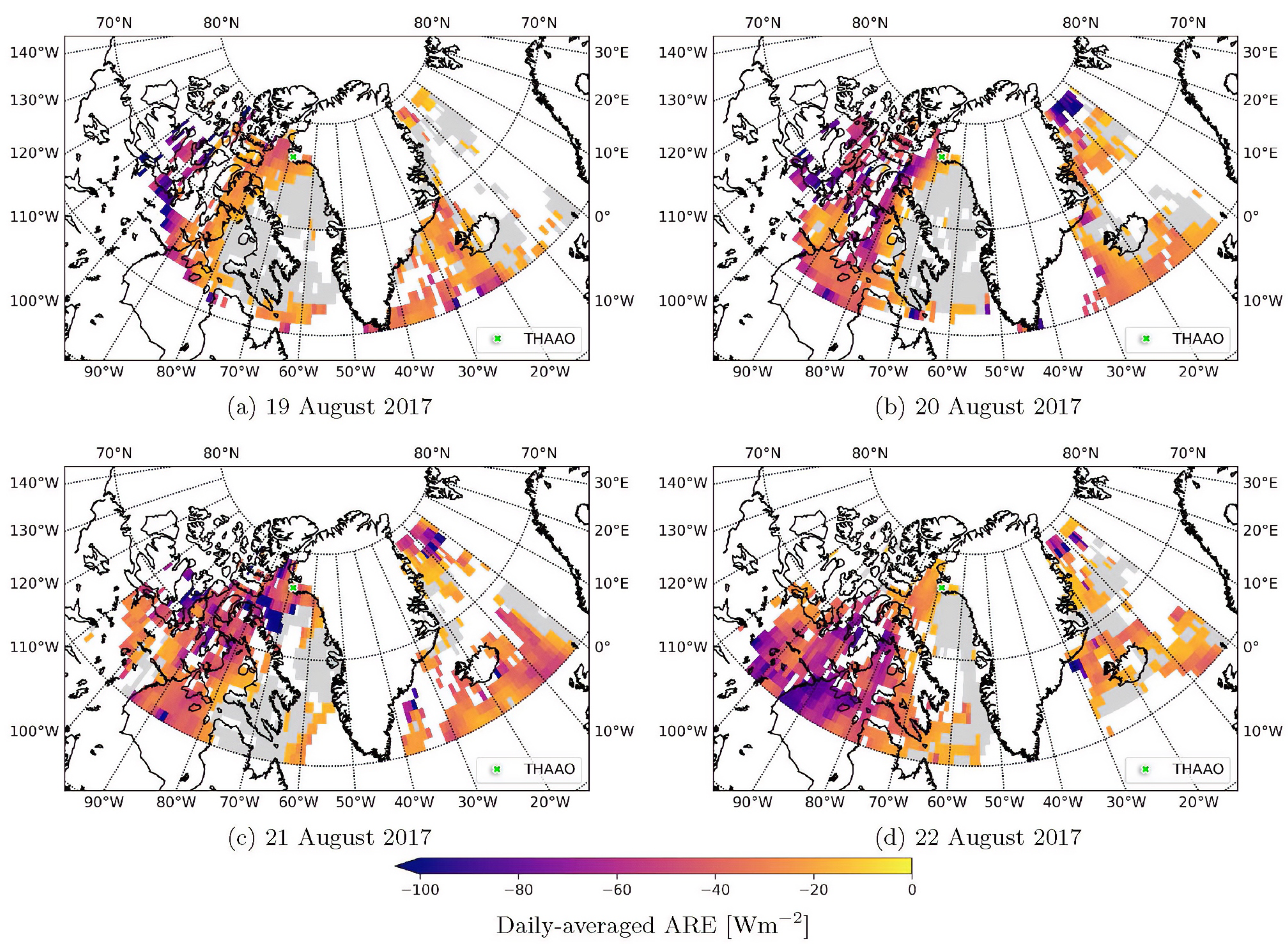
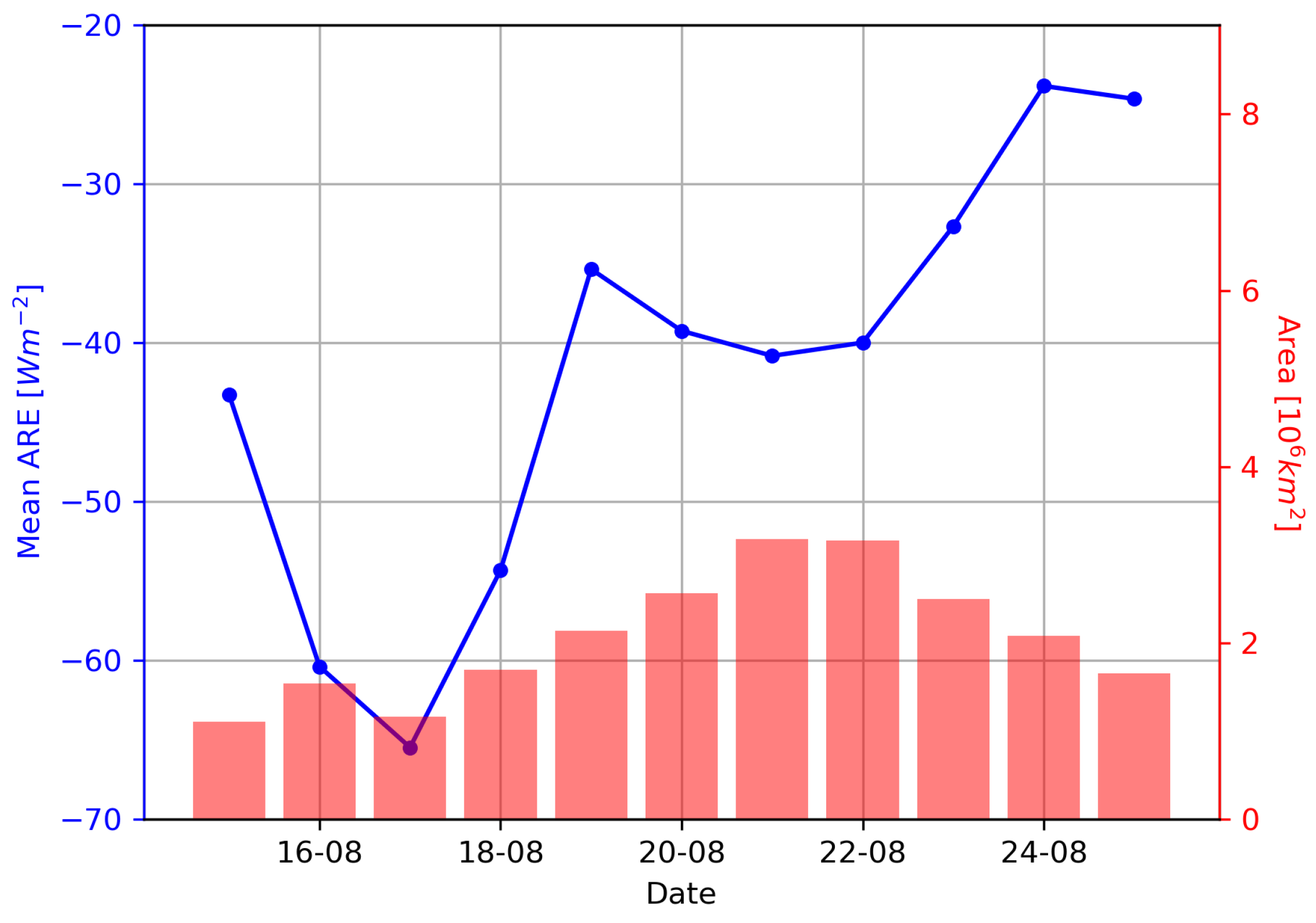
3.4. Radiative Impact over Western Arctic

The MODTRAN input parameters that produce the best agreement between simulated and measured SW↓ irradiances at THAAO were employed to simulate the values of AREE depicted in Figure 4 as a function of SZA and albedo. Using these AREE values together with albedo (Figure S4) and AOD values from MODIS, we spatially extended the estimates of the summer 2017 wildfires plume radiative impact over a broader Arctic area.
We investigated the distribution of AOD values measured at THAAO in August over an 11-year time span (2007–2019, excluding 2017, because it is considered in this study, and 2016, during which data were unavailable), and found that the 90th percentile of the long-term observations has an AOD value of 0.17. We then assumed that during the August 2017 event, which occurred in a season generally characterized by low AOD levels, only regions with AOD > 0.17 were directly affected by the smoke plume. The calculations of ARE were thus performed only over these areas.
Figure 5 shows the MODIS daily values of AOD at 550 nm. The grey-shaded areas represent pixels with AOD values below the 90th percentile threshold value (0.17). White areas represent pixels where no MODIS AOD data were available. Figure 6 shows the daily ARE spatial distribution obtained for the investigated area. An additional set of AOD and ARE spatial distribution maps between 15 and 18 August and between 23 and 25 August are shown in Figures S7 and S8.
MODIS visible images (Figure 1), EPIC [56], and OMPS [57] data indicate that the smoke plume gradually covered the northern part of Greenland, crossing the island from west to east during 18–22 August. We define the ARE daily regional mean as the average of the daily pixel values (Figure 6) throughout the area with AOD larger than the selected threshold (0.17) and within the geographical domain from 60 N to 80 N and from 110 W to 0 E. In Figure 7, the time series of the mean ARE values are plotted next to the area influenced by the plume. Since MODIS pixels represent areas of different extent depending on latitude, the ARE daily regional mean was calculated by weighting the ARE for the corresponding pixel area. From 15 to 25 August, the obtained daily regional mean values vary between −64.8 and −23.8 Wm 2 . The negative peak reached between 16 and 18 August corresponds to very high values of AOD in the western and southwestern corner of the domain (Nunavut, Manitoba, and Hudson Bay).
It is also worth noticing the large ARE values (∼−180 Wm 2 ) that are found much further away from the source regions, by the northeastern coast of Greenland, on 20–22 August. This result is in agreement with what is found by Zielinski et al. [24]. We estimated a peak of −127.5 TW for the cumulative ARE (obtained by multiplying the regional daily mean value by the area affected by the plume) on 21 and 22 August.
The mean and cumulative daily ARE values are affected by the Arctic area over which these estimates are calculated (see Figure 6). It varies from day to day, depending on the distribution of the smoke plume and on MODIS AOD data availability, which in turn depends on the cloud coverage. The area where we find an evidence of the influence of BB aerosol ranges from ∼1.1 to ∼ 3.1 × 10 6 km 2 , where the overall domain considered is approximately 9 × 10 6 km 2 . Given that MODIS AOD data are only available on ocean and ice-free land surfaces, our estimated cumulative ARE values are likely to be a lower limit of the actual surface cooling caused by the advection of BB aerosols over the Arctic. This is also supported by the results illustrated in Section 3.5.

3.5. Radiative Impact over the Greenland Ice Sheet (GIS)

By observing large AOD values over the Greenland Sea (Figure 5) and given MODIS, EPIC, and OMPS data during the 20–22 August period, we understand that the plume affected a large portion of northern Greenland which we did not account for in our calculations, as MODIS does not provide AOD measurements over the Greenland Ice Sheet (GIS).
To provide a rough estimate for this additional cooling at the surface, we calculated ARE values over the GIS (approximated as a plane located at 2500 m asl). Moreover, the ARE is calculated at sea level (SL, 0 m asl) to evaluate the effect due to altitude. The same surface albedo of 0.8 and the maximum value of AOD measured at THAAO in the considered period (0.86) are employed for these calculations. Results are given in Table 4 and show that ARE SL and GIS values are very similar for lower SZAs, that their difference increases with increasing SZA, and that larger negative ARE values are obtained at higher elevations.
As expected from Figure 4, Table 4 shows that the ARE due to the smoke plume over surfaces with large albedo (e.g., the GIS) is relatively small. The GIS accounts for approximately ∼ 0.5 × 10 6 km 2 , which could be added to the ∼ 3.1 × 10 6 km 2 of total considered surface on 21 August. The contribution from the GIS would lower the regional mean ARE (Figure 7) from −40.7 to −37.9 Wm 2 and add −9 TW to the estimated cumulative regional ARE of −127.5 TW. It is worth mentioning that these estimates also consider contributions from aerosol present in the southeastern corner of the domain (see Figure 6), which may be attributed to the Canadian and Greenlandic wildfires.

4. Conclusions

Arctic fires have been increasing during the recent summer seasons. Among the many impacts, the smoke plumes affect the surface radiation and energy budget. Additionally, local warming due to smoke aerosol absorption of solar radiation and surface cooling may favor an increase in the atmospheric vertical stability, leading to the suppression of cloud formation (e.g., Stone et al. [54]). In this study, we quantified the direct radiative effect in the Arctic using a representative case of the plumes transported over northern Greenland produced by the August 2017 wildfires in Canada and Greenland. This event reached the Thule High Arctic Atmospheric Observatory (THAAO, 76.53 N, 68.74 W, [23]) and large parts of the Arctic during 15–25 August 2017. We used a set of instruments available at THAAO to characterize the biomass-burning (BB) plume effects on atmospheric composition, and through modeling and satellite retrievals, we assessed the radiative impact at local and regional scales.
The analysis of PM 10 compounds shows a general increase in concentration of the BB markers during 14–25 August 2017. The enrichment in carboxylic acid, along with the HYSPLIT back-trajectories, suggests that the BB aerosols observed at THAAO originated from wildfires burning in northern Canada and south-western Greenland.
The MODTRAN6.0 radiative transfer model was used to estimate the aerosol radiative effect (ARE) and heating rate (AHR) vertical profiles at the THAAO. Instantaneous aerosol optical properties were constrained by a radiation closure study based on the net SW irradiance observations made at THAAO. The shortwave ARE at the surface was −43.7 Wm 2 at 78 solar zenith angle (SZA) for A O D = 0.63 . The peak aerosol heating rate (+0.50 K/day) was reached within the aerosol layer between 8 and 12 km altitude, while the maximum ARE (−45.4 Wm 2 ) was found at 3 km altitude, below the thickest aerosol layer. The smoke particles were detected by CALIPSO up to 12 km altitude in the region around THAAO, reaching the lower stratosphere (see Figure 3, EPIC and OMPS). Due to a combination of effects, the lower stratospheric region is expected to have undergone the strongest heating induced by aerosol. The MODTRAN model was also used to simulate the aerosol radiative effect efficiency (AREE) for different surface albedo and solar illumination in a region between 60 N and 80 N, 110 W and 0 E. The values of AREE span from −3 to −132 Wm 2 AOD 1 , depending on surface albedo and SZA, assuming the same aerosol optical properties of the instantaneous RT model calculations. Level-3 MODIS retrievals were employed to obtain AOD and surface albedo values in the region of interest to evaluate the mean daily ARE values.
The fire plume covered a vast portion of the Arctic, with particularly large AOD values occurring over northern Canada during the first part of the period and reaching the eastern Greenlandic coast, with reductions in surface shortwave radiation lasting for a few days. From 15 to 25 August 2017, the mean daily ARE values calculated over the region influenced by BB aerosol are between −65 and −25 Wm 2 . In particular, we calculated a cumulative ARE during this period and found a negative peak of −127.5 TW on 21 August within the affected region of the Arctic of ∼ 3.1 × 10 6 km 2 . The Greenland Ice Sheet (GIS) with its ∼ 0.5 × 10 6 km 2 could have contributed an additional −9 TW on 21 August, but the lack of AOD measurements above the GIS makes the latter a rough estimate.
Since BB aerosols are produced and transported mainly in summer when a considerable portion of the surface is free of snow, their impact on the Arctic surface radiation budget may increase.
Further analyses are needed to better characterize aerosols originating from different sources (i.e., boreal forests or peat), different regions, (i.e., Canada versus Greenland), and different fire intensities and transport times and quantify the overall radiative effects in the Arctic region where data are lacking (e.g., bright areas). More work is also needed to investigate the indirect effects which may act in the shortwave and longwave portions of the electromagnetic spectrum. From a wider perspective, this analysis showed that should smoke aerosols be more frequent in the Arctic and have a broader spatial extent, the radiative impact may be relevant for the regional energy budget with consequences for atmospheric stability and cloud microphysics, thus influencing feedback mechanisms of the Arctic climate.

Supplementary Materials

The following supporting information can be downloaded at: https://www.mdpi.com/article/10.3390/rs14020313/s1.

Author Contributions

Conceptualization, D.M., S.B., A.G.d.S.; methodology, F.C.Q., D.M., G.M., T.D.I., V.C., S.B.; formal analysis, F.C.Q., D.M., T.D.I., V.C., S.B., A.G.d.S.; writing—original draft preparation, D.M., G.M., S.B., A.G.d.S.; writing—review and editing, all authors; funding acquisition, G.M., V.C., G.P. All authors have read and agreed to the published version of the manuscript.

Funding

This research was partially funded by the Italian Ministry of University and Research (MIUR) within the framework of OASIS-YOPP—Observations of the Arctic Stratosphere In Support of YOPP (PNRA 2016–2018); CLARA2—CLouds And Radiation in the Arctic and Antarctica (PNRA 2019–2021), and ECAPAC—Effects of changing albedo and precipitation on the Arctic climate (PRA 2021–2023). The work of F. Calì Quaglia and G. Muscari was also partially funded under the INGV environmental project MACMAP—A Multidisciplinary Analysis of Climate change indicators in the Mediterranean And Polar regions (2020–2023). The NCAR FTIR observation program at Thule, Greenland is supported under contract by the National Aeronautics and Space Administration (NASA). The National Center for Atmospheric Research (NCAR) is sponsored by the U.S. National Science Foundation (NSF). The Thule work is also supported by the NSF Office of Polar Programs (OPP).

Institutional Review Board Statement

Not applicable.

Informed Consent Statement

Not applicable.

Data Availability Statement

AERONET data used in this study are available from the website https://aeronet.gsfc.nasa.gov/new_web/aerosols.html (accessed on 6 January 2022). Analyses of daily ozone data from OMI were produced with the Giovanni online data system (https://giovanni.gsfc.nasa.gov/giovanni/, accessed on 6 January 2022), developed and maintained by the NASA GES DISC. The authors gratefully acknowledge the NOAA Air Resources Laboratory (ARL) for the provision of the HYSPLIT transport and dispersion model used in this publication. The HYSPLIT trajectories were calculated using the PySPLIT package [58] for Python v3.6. FTIR data are available from https://www-air.larc.nasa.gov/missions/ndacc/data.html?station=thule/ames/ftir/ (accessed on 6 January 2022). The CALIOP V4.10 data were obtained from the NASA Langley Research Center Atmospheric Science Data Center at: https://asdc.larc.nasa.gov/project/CALIPSO (accessed on 6 January 2022), NASA/LARC/SD/ASDC, 2016. CALIPSO Lidar Level 1B profile data, V4-10. Available at: https://doi.org/10.5067/CALIOP/CALIPSO/LID_L1-STANDARD-V4-10 (accessed on 6 January 2022). The MODIS data were obtained from the Land Processes Distributed Active Archive Center at https://lpdaac.usgs.gov/product_search/ (accessed on 6 January 2022). The Level-3 MODIS MCD43C3 Version 6 Bidirectional Reflectance Distribution Function and Albedo data are available at https://lpdaac.usgs.gov/products/mcd43a3v006/ (accessed on 6 January 2022). The Level-3 MODIS Atmosphere Daily Global Product MOD08 and MYD08 are available at https://modaps.modaps.eosdis.nasa.gov/services/about/products/c6/MOD08_D3.html (accessed on 6 January 2022) and https://modaps.modaps.eosdis.nasa.gov/services/about/products/c6/MYD08_D3.html (accessed on 6 January 2022), respectively.

Acknowledgments

We thank Brent N. Holben for valuable suggestions and comments on this paper. We thank Brent N. Holben (PI) and Nis Jespen (Site Manager) of the AERONET Project for their effort in establishing and maintaining the AERONET site in Thule. We wish to thank the Danish Meteorological Institute for support at the Thule site.

Conflicts of Interest

The authors declare no conflict of interest.

References

  1. Serreze, M.C.; Walsh, J.E.; Chapin, F.S.; Osterkamp, T.; Dyurgerov, M.; Romanovsky, V.; Oechel, W.C.; Morison, J.; Zhang, T.; Barry, R.G. Observational evidence of recent change in the northern high-latitude environment. Clim. Chang. 2000, 46, 159–207. [Google Scholar] [CrossRef]
  2. Box, J.E.; Res, E.; Box, J.E.; Colgan, W.T.; Christensen, T.R.; Schmidt, N.M.; Lund, M.; Parmentier, F.J.W.J.W.; Brown, R.; Bhatt, U.S.; et al. Key indicators of Arctic climate change: 1971–2017 Key indicators of Arctic climate change: 1971–2017. Environ. Res. Lett. 2019, 14, 045010. [Google Scholar] [CrossRef]
  3. Jolly, W.M.; Cochrane, M.A.; Freeborn, P.H.; Holden, Z.A.; Brown, T.J.; Williamson, G.J.; Bowman, D.M.J.S. Climate-induced variations in global wildfire danger from 1979 to 2013. Nat. Commun. 2015, 6, 7537. [Google Scholar] [CrossRef]
  4. Masrur, A.; Petrov, A.N.; DeGroote, J. Circumpolar spatio-temporal patterns and contributing climatic factors of wildfire activity in the Arctic tundra from 2001–2015. Environ. Res. Lett. 2018, 13, 014019. [Google Scholar] [CrossRef] [Green Version]
  5. Bret-Harte, M.S.; Mack, M.C.; Shaver, G.R.; Huebner, D.C.; Johnston, M.; Mojica, C.A.; Pizano, C.; Reiskind, J.A. The response of Arctic vegetation and soils following an unusually severe tundra fire. Philos. Trans. R. Soc. B Biol. Sci. 2013, 368, 20120490. [Google Scholar] [CrossRef]
  6. Wang, C.; Wang, Z.; Kong, Y.; Zhang, F.; Yang, K.; Zhang, T. Most of the Northern Hemisphere Permafrost Remains under Climate Change. Sci. Rep. 2019, 9, 3295. [Google Scholar] [CrossRef] [Green Version]
  7. Schuur, E.A.G.; Bockheim, J.; Canadell, J.G.; Euskirchen, E.; Field, C.B.; Goryachkin, S.V.; Hagemann, S.; Kuhry, P.; Lafleur, P.M.; Lee, H.; et al. Vulnerability of Permafrost Carbon to Climate Change: Implications for the Global Carbon Cycle. BioScience 2008, 58, 701–714. [Google Scholar] [CrossRef]
  8. McGuire, A.D.; Anderson, L.G.; Christensen, T.R.; Dallimore, S.; Guo, L.; Hayes, D.J.; Heimann, M.; Lorenson, T.D.; Macdonald, R.W.; Roulet, N. Sensitivity of the carbon cycle in the Arctic to climate change. Ecol. Monogr. 2009, 79, 523–555. [Google Scholar] [CrossRef] [Green Version]
  9. Young, A.M.; Higuera, P.E.; Duffy, P.A.; Hu, F.S. Climatic thresholds shape northern high-latitude fire regimes and imply vulnerability to future climate change. Ecography 2017, 40, 606–617. [Google Scholar] [CrossRef]
  10. Higuera, P.E.; Brubaker, L.B.; Anderson, P.M.; Brown, T.A.; Kennedy, A.T.; Hu, F.S. Frequent Fires in Ancient Shrub Tundra: Implications of Paleorecords for Arctic Environmental Change. PLoS ONE 2008, 3, e0001744. [Google Scholar] [CrossRef]
  11. Yue, X.; Mickley, L.J.; Logan, J.A.; Hudman, R.C.; Martin, M.V.; Yantosca, R.M. Impact of 2050 climate change on North American wildfire: Consequences for ozone air quality. Atmos. Chem. Phys. 2015, 15, 10033–10055. [Google Scholar] [CrossRef] [Green Version]
  12. Markowicz, K.; Lisok, J.; Xian, P. Simulations of the effect of intensive biomass burning in July 2015 on Arctic radiative budget. Atmos. Environ. 2017, 171, 248–260. [Google Scholar] [CrossRef]
  13. Evangeliou, N.; Kylling, A.; Eckhardt, S.; Myroniuk, V.; Stebel, K.; Paugam, R.; Zibtsev, S.; Stohl, A. Open fires in Greenland in summer 2017: Transport, deposition and radiative effects of BC, OC and BrC emissions. Atmos. Chem. Phys. 2019, 19, 1393–1411. [Google Scholar] [CrossRef] [Green Version]
  14. Veraverbeke, S.; Rogers, B.M.; Goulden, M.L.; Jandt, R.R.; Miller, C.E.; Wiggins, E.B.; Randerson, J.T. Lightning as a major driver of recent large fire years in North American boreal forests. Nat. Clim. Chang. 2017, 7, 529–534. [Google Scholar] [CrossRef]
  15. Kasischke, E.S.; Turetsky, M.R. Recent changes in the fire regime across the North American boreal region—Spatial and temporal patterns of burning across Canada and Alaska. Geophys. Res. Lett. 2006, 33, 437–451. [Google Scholar] [CrossRef] [Green Version]
  16. Kharuk, V.I.; Ponomarev, E.I. Spatiotemporal characteristics of wildfire frequency and relative area burned in larch-dominated forests of Central Siberia. Russ. J. Ecol. 2017, 48, 507–512. [Google Scholar] [CrossRef]
  17. Kharuk, V.I.; Ponomarev, E.I.; Ivanova, G.A.; Dvinskaya, M.L.; Coogan, S.C.P.; Flannigan, M.D. Wildfires in the Siberian taiga. Ambio 2021, 50, 1953–1974. [Google Scholar] [CrossRef]
  18. Balshi, M.S.; McGuire, A.D.; Duffy, P.; Flannigan, M.; Walsh, J.; Melillo, J. Assessing the response of area burned to changing climate in western boreal North America using a Multivariate Adaptive Regression Splines (MARS) approach. Glob. Chang. Biol. 2009, 15, 578–600. [Google Scholar] [CrossRef]
  19. Flannigan, M.D.; Wotton, B.M.; Marshall, G.A.; de Groot, W.J.; Johnston, J.; Jurko, N.; Cantin, A.S. Fuel moisture sensitivity to temperature and precipitation: Climate change implications. Clim. Chang. 2016, 134, 59–71. [Google Scholar] [CrossRef]
  20. Scholten, R.C.; Jandt, R.; Miller, E.A.; Rogers, B.M.; Veraverbeke, S. Overwintering fires in boreal forests. Nature 2021, 593, 399–404. [Google Scholar] [CrossRef]
  21. McCarty, J.L.; Smith, T.E.L.; Turetsky, M.R. Arctic fires re-emerging. Nat. Geosci. 2020, 13, 658–660. [Google Scholar] [CrossRef]
  22. Lutsch, E.; Strong, K.; Jones, D.B.; Blumenstock, T.; Conway, S.; Fisher, J.A.; Hannigan, J.W.; Hase, F.; Kasai, Y.; Mahieu, E.; et al. Detection and attribution of wildfire pollution in the Arctic and northern midlatitudes using a network of Fourier-Transform infrared spectrometers and GEOS-Chem. Atmos. Chem. Phys. 2020, 20, 12813–12851. [Google Scholar] [CrossRef]
  23. Thule High Arctic Atmospheric Observatory (THAAO). Available online: https://www.thuleatmos-it.it/ (accessed on 29 November 2021).
  24. Zielinski, T.; Bolzacchini, E.; Cataldi, M.; Ferrero, L.; Graßl, S.; Hansen, G.; Mateos, D.; Mazzola, M.; Neuber, R.; Pakszys, P.; et al. Study of chemical and optical properties of biomass burning aerosols during long-range transport events toward the arctic in summer 2017. Atmosphere 2020, 11, 84. [Google Scholar] [CrossRef] [Green Version]
  25. Peterson, D.A.; Campbell, J.R.; Hyer, E.J.; Fromm, M.D.; Kablick, G.P.; Cossuth, J.H.; DeLand, M.T. Wildfire-driven thunderstorms cause a volcano-like stratospheric injection of smoke. npj Clim. Atmos. Sci. 2018, 1, 30. [Google Scholar] [CrossRef] [PubMed] [Green Version]
  26. Christian, K.; Yorks, J.; Das, S. Differences in the evolution of pyrocumulonimbus and volcanic stratospheric plumes as observed by cats and caliop space-based lidars. Atmosphere 2020, 11, 1035. [Google Scholar] [CrossRef]
  27. Das, S.; Colarco, P.R.; Oman, L.D.; Taha, G.; Torres, O. The long-term transport and radiative impacts of the 2017 British Columbia pyrocumulonimbus smoke aerosols in the stratosphere. Atmos. Chem. Phys. 2021, 21, 12069–12090. [Google Scholar] [CrossRef]
  28. Ansmann, A.; Baars, H.; Chudnovsky, A.; Mattis, I.; Veselovskii, I.; Haarig, M.; Seifert, P.; Engelmann, R.; Wandinger, U. Extreme levels of Canadian wildfire smoke in the stratosphere over central Europe on 21–22 August 2017. Atmos. Chem. Phys. 2018, 18, 11831–11845. [Google Scholar] [CrossRef] [Green Version]
  29. Lutsch, E.; Strong, K.; Jones, D.B.A.; Ortega, I.; Hannigan, J.W.; Dammers, E.; Shephard, M.W.; Morris, E.; Murphy, K.; Evans, M.J.; et al. Unprecedented Atmospheric Ammonia Concentrations Detected in the High Arctic From the 2017 Canadian Wildfires. J. Geophys. Res. Atmos. 2019, 124, 8178–8202. [Google Scholar] [CrossRef]
  30. Haarig, M.; Ansmann, A.; Baars, H.; Jimenez, C.; Veselovskii, I.; Engelmann, R.; Althausen, D. Depolarization and lidar ratios at 355, 532, and 1064 nm and microphysical properties of aged tropospheric and stratospheric Canadian wildfire smoke. Atmos. Chem. Phys. 2018, 18, 11847–11861. [Google Scholar] [CrossRef] [Green Version]
  31. Di Sarra, A.; Cacciani, M.; Di Girolamo, P.; Fiocco, G.; Fuà, D.; Knudsen, B.; Larsen, N.; Joergensen, T.S. Observations of correlated behavior of stratospheric ozone and aerosol at Thule during winter 1991–1992. Geophys. Res. Lett. 1992, 19, 1823–1826. [Google Scholar] [CrossRef]
  32. Hannigan, J.W.; Coffey, M.T.; Goldman, A. Semiautonomous FTS Observation System for Remote Sensing of Stratospheric and Tropospheric Gases. J. Atmos. Ocean. Technol. 2009, 26, 1814–1828. [Google Scholar] [CrossRef]
  33. Network for the Detection of Atmospheric Composition Change (NDACC). Available online: ndacc-uvvis-wg.aeronomie.be/tools/NDACC_UVVIS-WG_NO2settings_v4.pdf (accessed on 1 December 2021).
  34. Holben, B.; Eck, T.; Slutsker, I.; Tanré, D.; Buis, J.; Setzer, A.; Vermote, E.; Reagan, J.; Kaufman, Y.; Nakajima, T.; et al. AERONET—A Federated Instrument Network and Data Archive for Aerosol Characterization. Remote Sens. Environ. 1998, 66, 1–16. [Google Scholar] [CrossRef]
  35. Smirnov, A.; Holben, B.N.; Eck, T.F.; Dubovik, O.; Slutsker, I. Cloud-screening and quality control algorithms for the AERONET database. Remote Sens. Environ. 2000, 73, 337–349. [Google Scholar] [CrossRef]
  36. Giles, D.M.; Sinyuk, A.; Sorokin, M.G.; Schafer, J.S.; Smirnov, A.; Slutsker, I.; Eck, T.F.; Holben, B.N.; Lewis, J.R.; Campbell, J.R.; et al. Advancements in the Aerosol Robotic Network (AERONET) Version 3 database–automated near-real-time quality control algorithm with improved cloud screening for Sun photometer aerosol optical depth (AOD) measurements. Atmos. Meas. Tech. 2019, 12, 169–209. [Google Scholar] [CrossRef] [Green Version]
  37. Mateos, D.; Pace, G.; Meloni, D.; Bilbao, J.; di Sarra, A.; de Miguel, A.; Casasanta, G.; Min, Q. Observed influence of liquid cloud microphysical properties on ultraviolet surface radiation. J. Geophys. Res. Atmos. 2014, 119, 2429–2440. [Google Scholar] [CrossRef]
  38. Becagli, S.; Caiazzo, L.; Di Iorio, T.; di Sarra, A.; Meloni, D.; Muscari, G.; Pace, G.; Severi, M.; Traversi, R. New insights on metals in the Arctic aerosol in a climate changing world. Sci. Total Environ. 2020, 741, 140511. [Google Scholar] [CrossRef]
  39. Winker, D.M.; Pelon, J.R.; McCormick, M.P. The CALIPSO mission: Spaceborne lidar for observation of aerosols and clouds. In Lidar Remote Sensing for Industry and Environment Monitoring III; International Society for Optics and Photonics: Bellingham, WA, USA, 2003. [Google Scholar] [CrossRef] [Green Version]
  40. Burton, S.P.; Ferrare, R.A.; Hostetler, C.A.; Hair, J.W.; Rogers, R.R.; Obland, M.D.; Butler, C.F.; Cook, A.L.; Harper, D.B.; Froyd, K.D. Aerosol classification using airborne High Spectral Resolution Lidar measurements—Methodology and examples. Atmos. Meas. Tech. 2012, 5, 73–98. [Google Scholar] [CrossRef] [Green Version]
  41. Platnick, S.; King, M.; Hubanks, P. MODIS Atmosphere L3 Daily Product; NASA MODIS Adaptive Processing System, Goddard Space Flight Center: Greenbelt, MD, USA, 2015. [Google Scholar] [CrossRef]
  42. Schaaf, C.; Wang, Z. MCD43A3 MODIS/Terra+Aqua BRDF/Albedo Daily L3 Global—500 m V006 [Data Set]; USGS: Sioux Falls, SD, USA, 2015. [Google Scholar] [CrossRef]
  43. Jin, Z.; Charlock, T.P.; Smith, W.L.; Rutledge, K. A parameterization of ocean surface albedo. Geophys. Res. Lett. 2004, 31, 1–4. [Google Scholar] [CrossRef]
  44. Berk, A.; Conforti, P.; Kennett, R.; Perkins, T.; Hawes, F.; van den Bosch, J. MODTRAN6: A major upgrade of the MODTRAN radiative transfer code. In Algorithms and Technologies for Multispectral, Hyperspectral, and Ultraspectral Imagery; SPIE: Bellingham, WA, USA, 2014. [Google Scholar] [CrossRef]
  45. McClatchey, R.A.; Fenn, R.; Selby, J.; Volz, F.; Garing, J. Optical Properties of the Atmosphere, 3rd ed.; Environmental Research Papers; Air Force Systems Command, United States Air Force: Baltimore, MD, USA, 1972; Volume 411, p. 108. [Google Scholar]
  46. Dirksen, R.; Dobber, M.; Voors, R.; Levelt, P. Prelaunch characterization of the Ozone Monitoring Instrument transfer function in the spectral domain. Appl. Opt. 2006, 45, 3972. [Google Scholar] [CrossRef]
  47. Dubovik, O.; Holben, B.; Eck, T.F.; Smirnov, A.; Kaufman, Y.J.; King, M.D.; Tanré, D.; Slutsker, I. Variability of absorption and optical properties of key aerosol types observed in worldwide locations. J. Atmos. Sci. 2002, 59, 590–608. [Google Scholar] [CrossRef]
  48. Zhuravleva, T.B.; Kabanov, D.M.; Nasrtdinov, I.M.; Russkova, T.V.; Sakerin, S.M.; Smirnov, A.; Holben, B.N. Radiative characteristics of aerosol during extreme fire event over Siberia in Summer 2012. Atmos. Meas. Tech. 2017, 10, 179–198. [Google Scholar] [CrossRef] [Green Version]
  49. Riihelä, A.; King, M.D.; Anttila, K. The surface albedo of the Greenland Ice Sheet between 1982 and 2015 from the CLARA-A2 dataset and its relationship to the ice sheet’s surface mass balance. Cryosphere 2019, 13, 2597–2614. [Google Scholar] [CrossRef] [Green Version]
  50. Viatte, C.; Strong, K.; Hannigan, J.; Nussbaumer, E.; Emmons, L.K.; Conway, S.; Paton-Walsh, C.; Hartley, J.; Benmergui, J.; Lin, J. Identifying fire plumes in the Arctic with tropospheric FTIR measurements and transport models. Atmos. Chem. Phys. 2015, 15, 2227–2246. [Google Scholar] [CrossRef] [Green Version]
  51. Moroni, B.; Cappelletti, D.; Crocchianti, S.; Becagli, S.; Caiazzo, L.; Traversi, R.; Udisti, R.; Mazzola, M.; Markowicz, K.; Ritter, C.; et al. Morphochemical characteristics and mixing state of long range transported wildfire particles at Ny-Ålesund (Svalbard Islands). Atmos. Environ. 2017, 156, 135–145. [Google Scholar] [CrossRef]
  52. Kalogridis, A.C.; Popovicheva, O.; Engling, G.; Diapouli, E.; Kawamura, K.; Tachibana, E.; Ono, K.; Kozlov, V.; Eleftheriadis, K. Smoke aerosol chemistry and aging of Siberian biomass burning emissions in a large aerosol chamber. Atmos. Environ. 2018, 185, 15–28. [Google Scholar] [CrossRef]
  53. Bowen, H.J.M. Environmental Chemistry of the Elements; Academic Press: London, UK; New York, NY, USA, 1979. [Google Scholar]
  54. Stone, R.S.; Anderson, G.P.; Shettle, E.P.; Andrews, E.; Loukachine, K.; Dutton, E.G.; Schaaf, C.; Roman, M.O. Radiative impact of boreal smoke in the Arctic: Observed and modeled. J. Geophys. Res. 2008, 113, D14S16. [Google Scholar] [CrossRef]
  55. Di Biagio, C.; di Sarra, A.; Eriksen, P.; Ascanius, S.E.; Muscari, G.; Holben, B. Effect of surface albedo, water vapour, and atmospheric aerosols on the cloud-free shortwave radiative budget in the Arctic. Clim. Dyn. 2012, 39, 953–969. [Google Scholar] [CrossRef]
  56. Earth Polychromatic Imaging Camera (EPIC) UVAI. Available online: https://epic.gsfc.nasa.gov/science/products/uv (accessed on 29 November 2021).
  57. Ozone Mapping and Profiler Suite (OMPS) UVAI. Available online: https://acd-ext.gsfc.nasa.gov/People/Seftor/OMPS_AI_August_2017.html (accessed on 29 November 2021).
  58. Warner, M.S. Introduction to PySPLIT: A Python Toolkit for NOAA ARL’s HYSPLIT Model. Comput. Sci. Eng. 2018, 20, 47–62. [Google Scholar] [CrossRef]
Figure 1. Terra-MODIS image for 24 August 2017. Red dots mark active fires individuated as “Fires and Thermal Anomalies”. Large fires were detected over Canada and smaller fires along the western coast of Greenland.
Remotesensing 14 00313 g001
Figure 2. Time series of chemical species and physical properties measured at the THAAO during August 2017. (a) Total, fine, and coarse AOD data (unitless) are obtained from AERONET Version 3 dataset at 500 nm. (b) SW↓ and PAR↓ are obtained from the pyranometer and quantum sensor, respectively. (c,e,g) H 2 CO, NH 3 , C 2 H 6 , HCN, and CO concentrations are obtained from FTIR measurements; for further details, see Section 2. (d,f,h) The concentrations of nssSO 4 2 , NH 4 + , nssK + , oxalate (Ox), glycolate (Gly), and Formate (For) were measured in PM 10 samples (48-h resolution).
Remotesensing 14 00313 g002
Figure 3. (a) Aerosol Radiative Effect (ARE) profiles for 21 August 2017 at S Z A = 78 calculated by using (b) the aerosol extinction profile derived from CALIOP and (c) Aerosol Heating Rate (AHR) profiles for 21 August 2017 S Z A = 78 .
Remotesensing 14 00313 g003
Figure 4. AREE as a function of SZA and surface albedo. See Section 3.3 for further details.
Remotesensing 14 00313 g004
Figure 5. MODIS daily AOD spatial distribution at 550 nm for 19–22 August 2017. The grey-shaded area represents pixels with AOD values below the 90th percentile threshold value (0.17). White areas represent pixels where no MODIS AOD data were available. See text for further details.
Remotesensing 14 00313 g005
Figure 6. The same as (Figure 5) but for daily-average ARE. White areas represent pixels where no MODIS AOD data were available or data were outside the considered domain. See text for further details.
Remotesensing 14 00313 g006
Figure 7. Time evolution of the ARE regional mean values (blue line) over the pixels available (transformed into an area, red bars) in the region considered (60°N–80°N, 110°W–0°E).
Remotesensing 14 00313 g007
Table 1. Summary of the single scattering albedo (SSA) and asymmetry factor (g) values from: column A = Dubovik et al. [47]; column B = Zhuravleva et al. [48]; column C = Zielinski et al. [24]. See text for details.
λ [nm]ABC
SSAgSSAgSSAg
4400.940.690.920.680.820.75
6700.9350.610.910.590.800.68
8700.920.550.890.550.740.63
10200.910.530.880.540.690.58
Table 2. Irradiances measured at THAAO on 17 and 21 August and their difference for S Z A = 78 and A O D = 0.63 ; all the values are in [Wm 2 ] except for AREE which are in [Wm 2 AOD 1 ].
17 August21 AugustDiff.AREE
SW↓175.1123.9−51.2 (−29.2%)
SW↑35.721.2−14.5 (−40.6%)−58.6
net SW139.4102.7−36.7
PAR↓70.246.2−24.0 (−34.2%)
PAR↑10.35.5−4.8 (−46.6%)−30.7
net PAR59.940.7−19.2
Table 3. Modeled SW irradiances (upward and downward) with the different aerosol optical properties found in the literature (Table 1, columns A, B, C) and comparison with ground-based measurements from 21 August 2017.
ABC
SW↑SW↓SW↑SW↓SW↑SW↓
Meas. [Wm 2 ]21.2123.921.2123.921.2123.9
Model [Wm 2 ]21.2122.520.5118.918.2105.7
Difference [%]0.0−1.1−3.3−4.0−14.2−14.7
Table 4. Comparison of ARE values over land at sea level (SL) and over the Greenland Ice Sheet (GIS) for different SZA at a constant albedo of 0.8 and AOD of 0.86. ARE values are in Wm 2 .
SZA [ ]455055606570758085
ARE GIS−12.9−15.1−17.4−19.5−21.3−22.2−21.7−19.0−13.4
ARE SL−13.0−14.7−16.2−17.6−18.5−18.6−17.3−14.3−9.2
ARE Diff.0.1−0.5−1.2−1.9−2.8−3.7−4.4−4.8−4.3
(GIS-SL)
Publisher’s Note: MDPI stays neutral with regard to jurisdictional claims in published maps and institutional affiliations.

