Water Quality Sustainability Evaluation under Uncertainty: A Multi-Scenario Analysis Based on Bayesian Networks


 , , and
Abstract
:1. Introduction
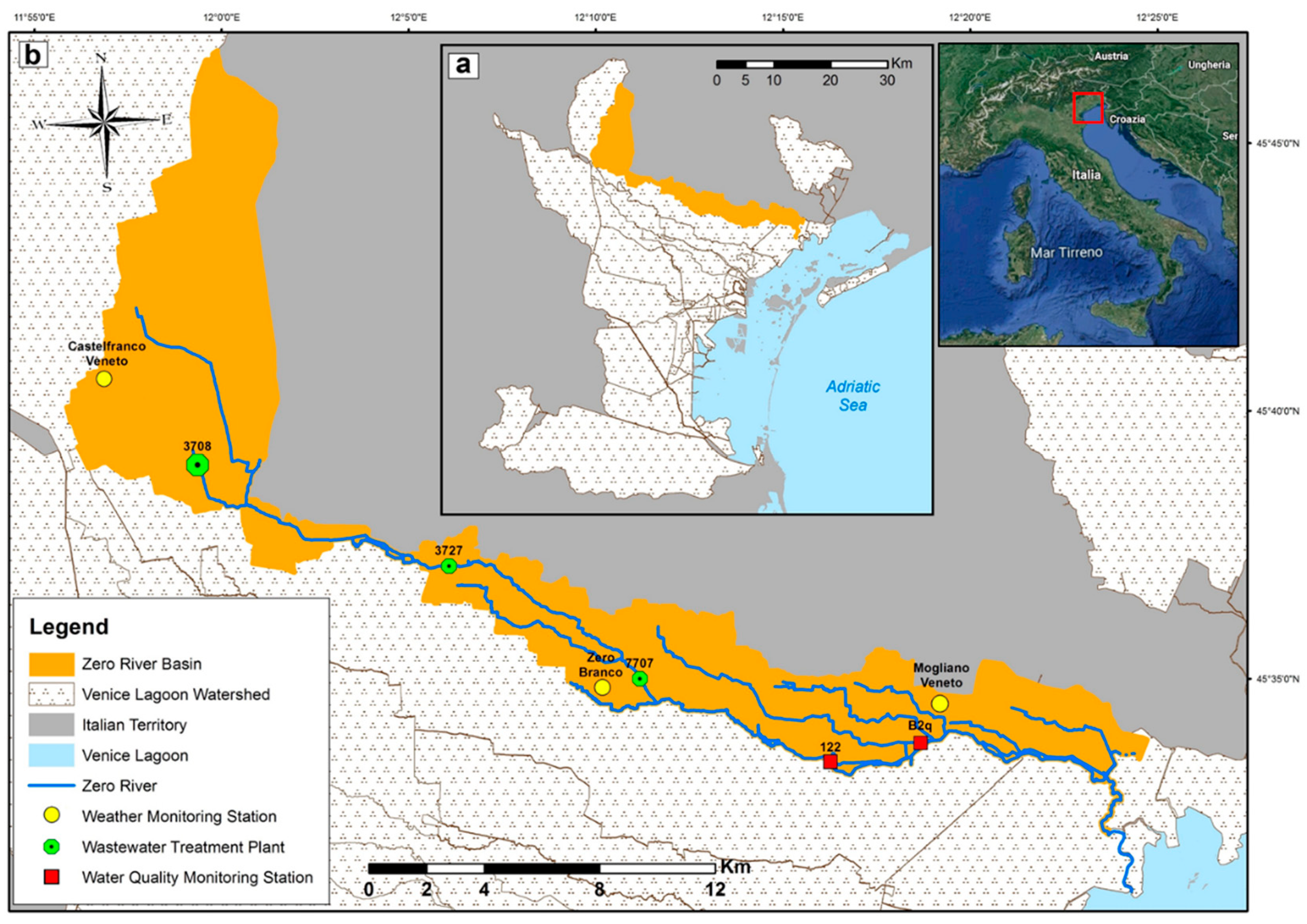
Study Area
2. Materials and Methods
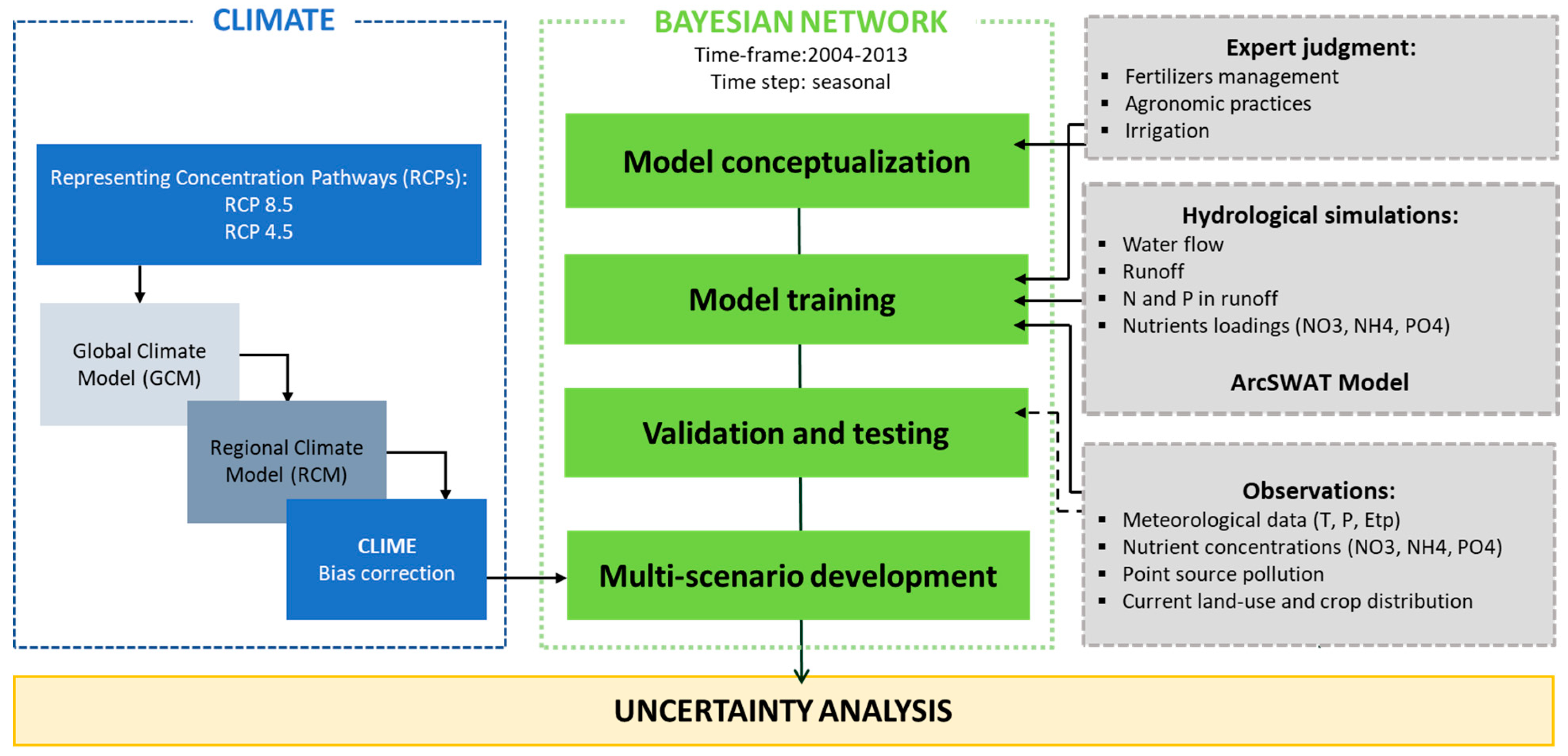
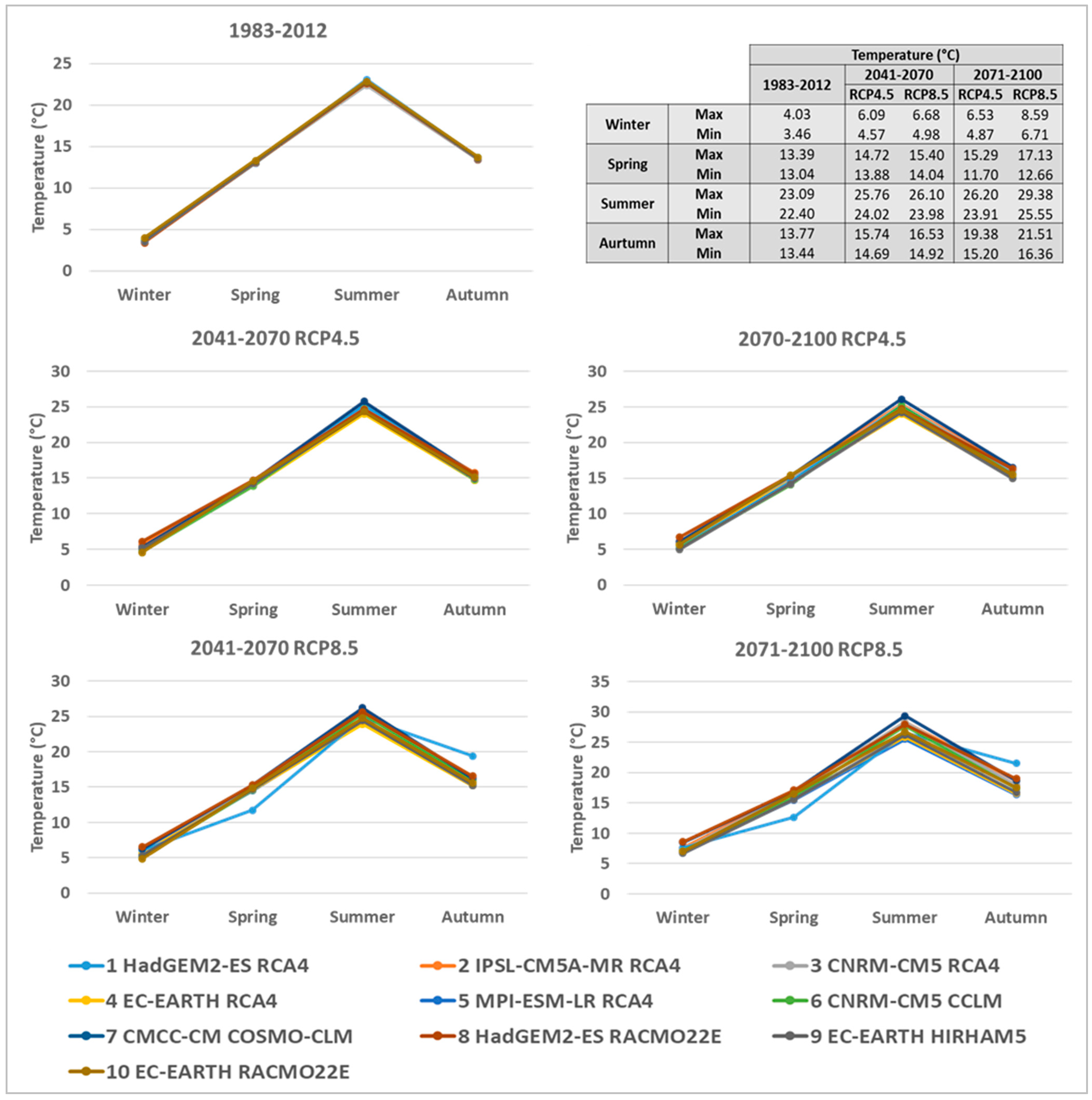
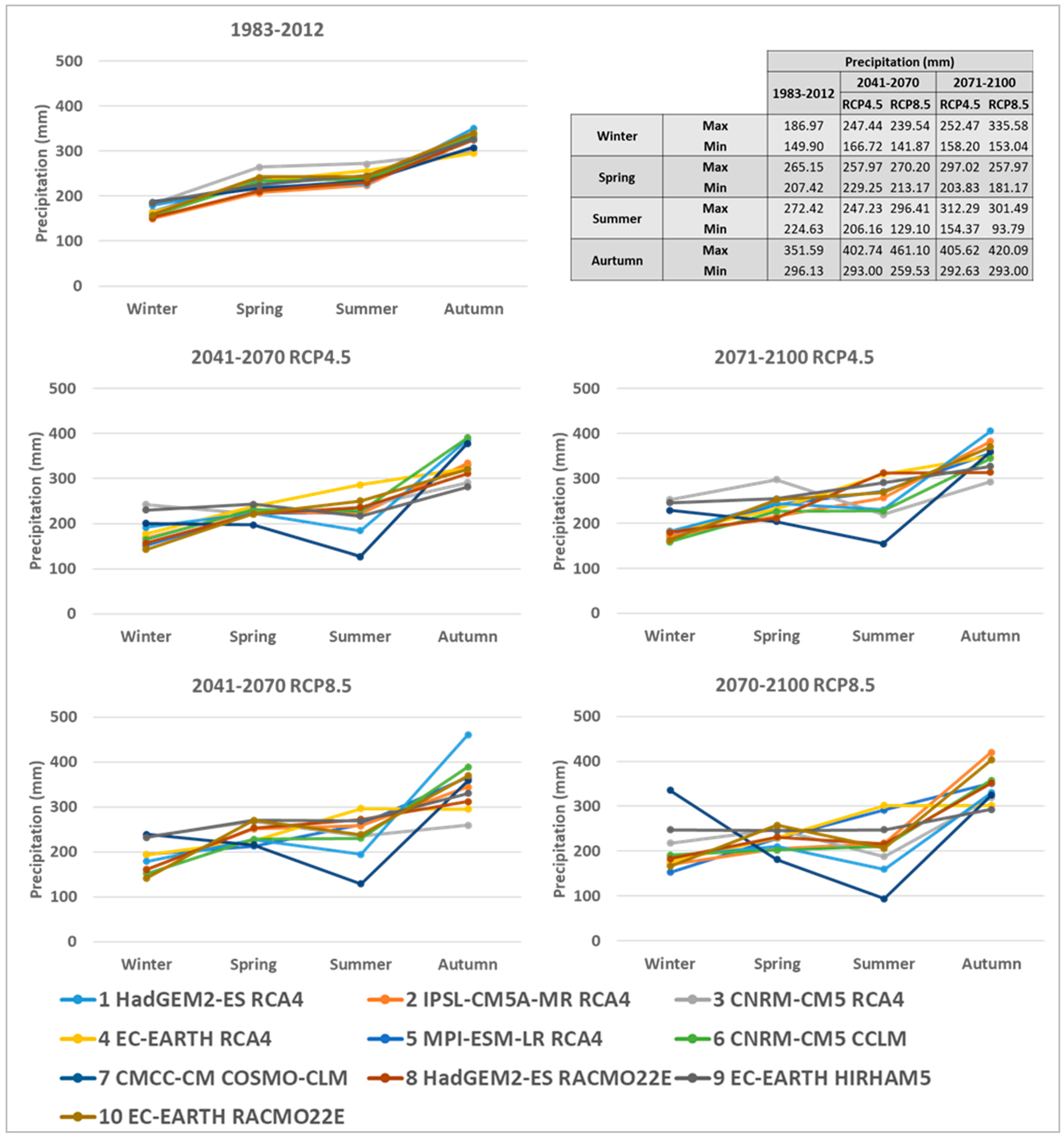
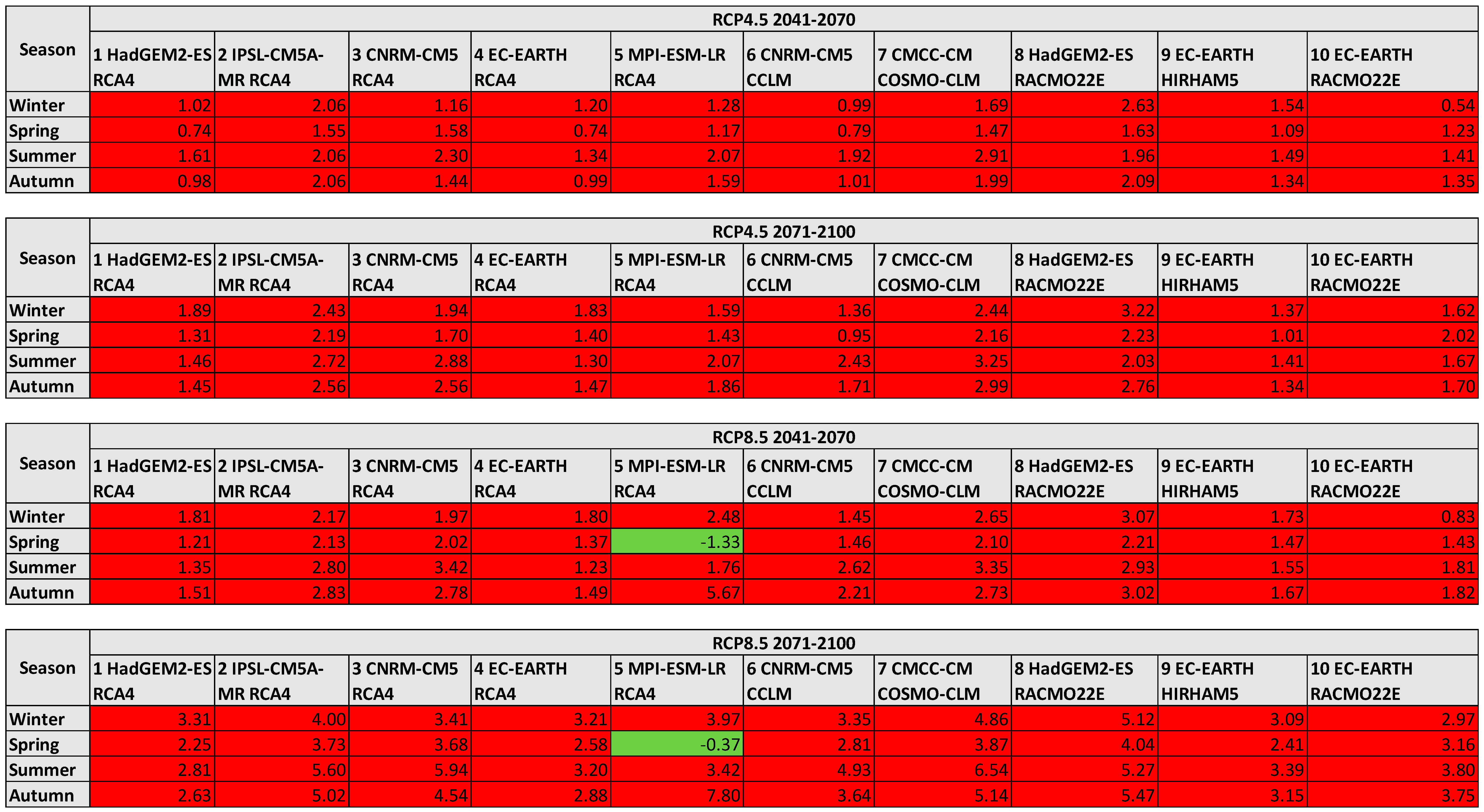
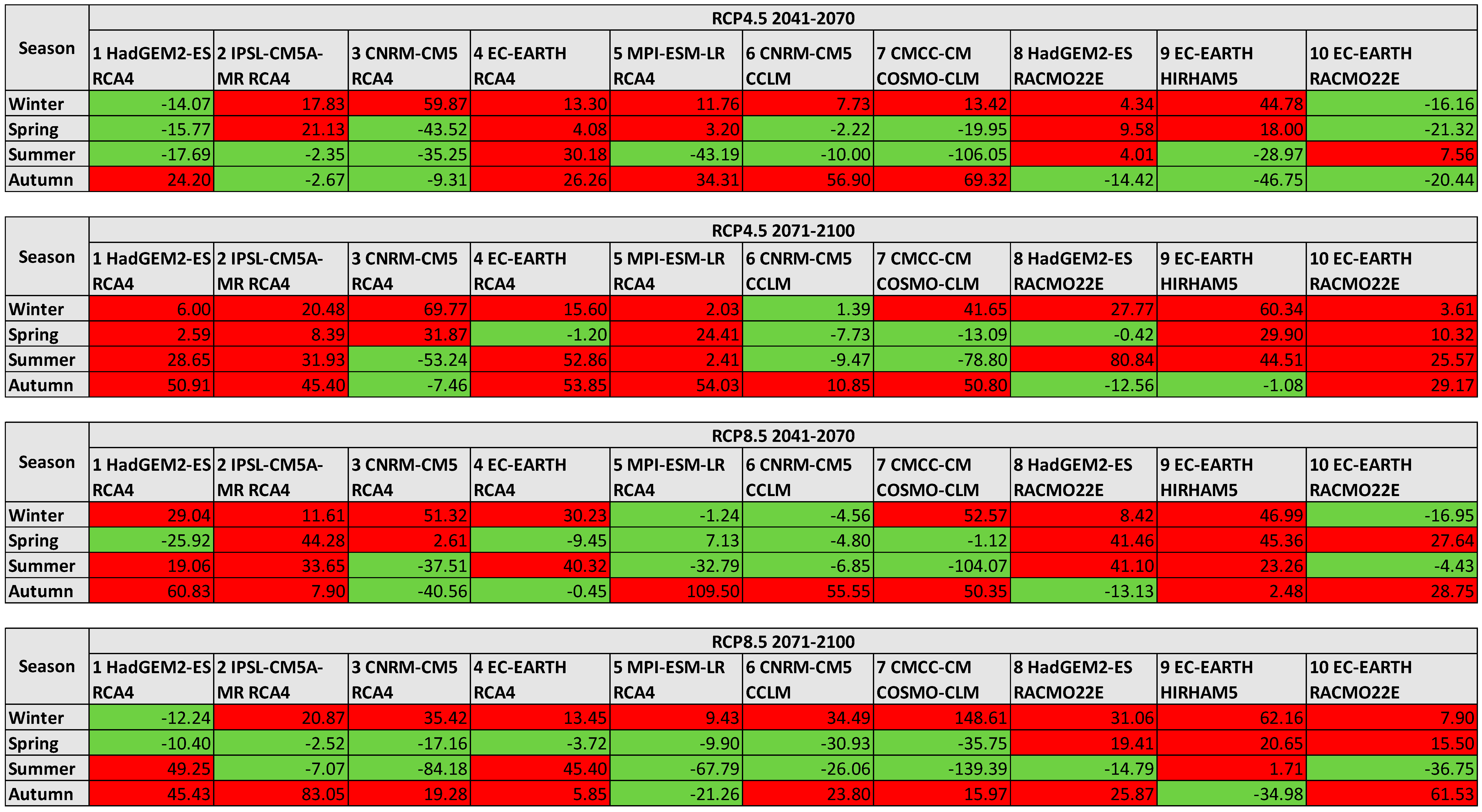
2.1. Climate Change Projections
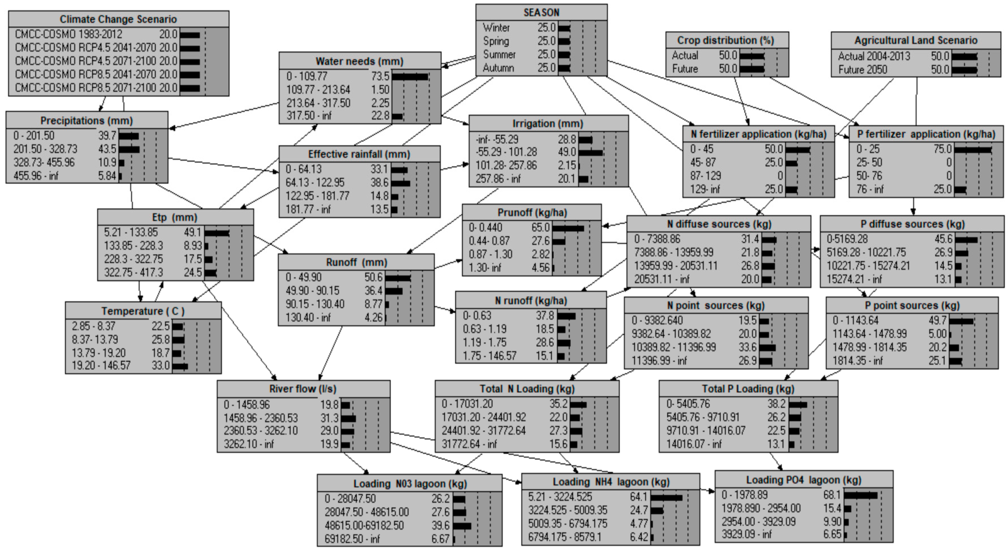
2.2. Bayesian Network Model
2.2.1. BN Development and Training
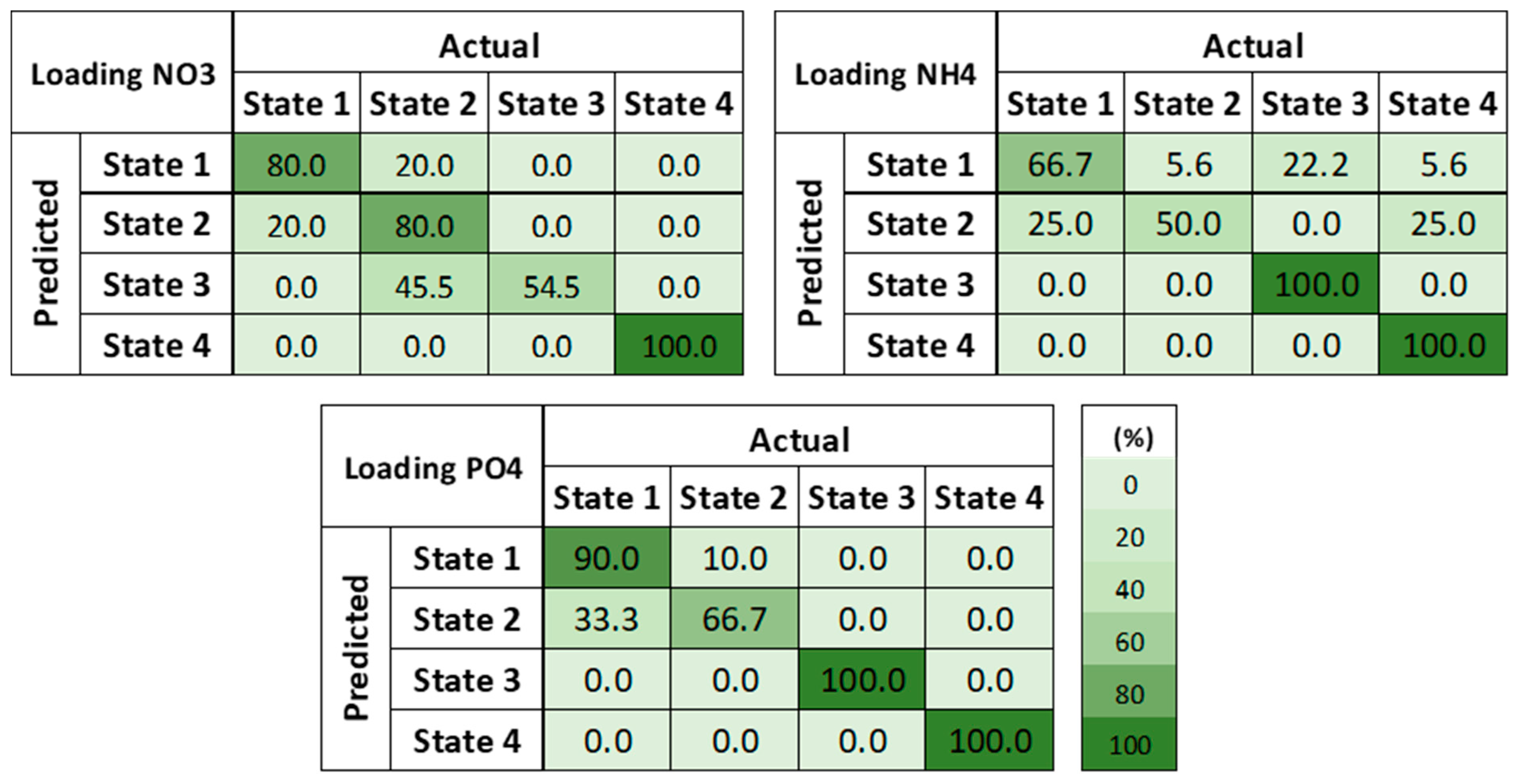
2.2.2. BN Evaluation
Predictive Accuracy
Sensitivity Analysis
2.2.3. Scenarios and Uncertainty Analysis
3. Results
3.1. BN Evaluation
3.1.1. Accuracy
3.1.2. Sensitivity Analysis
3.2. Climate Change Scenarios for the Zero River Basin
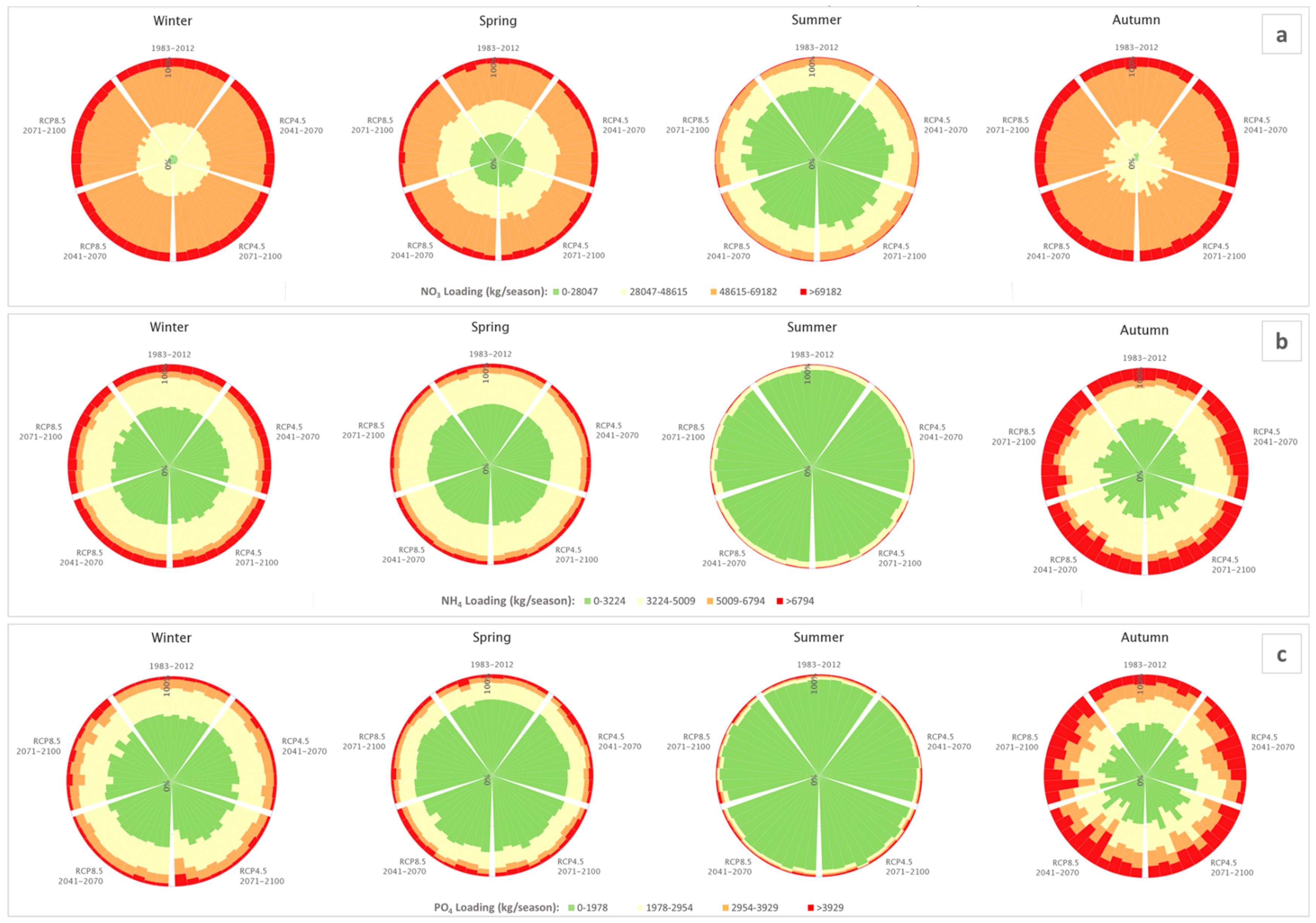
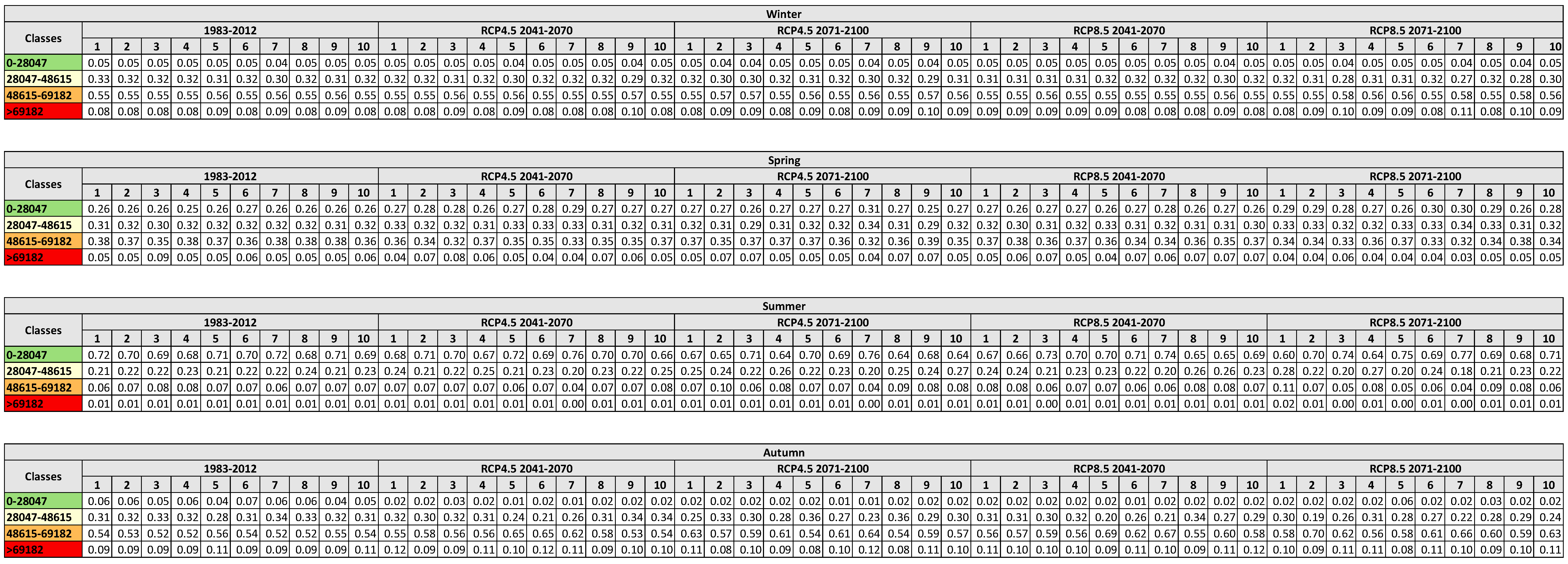
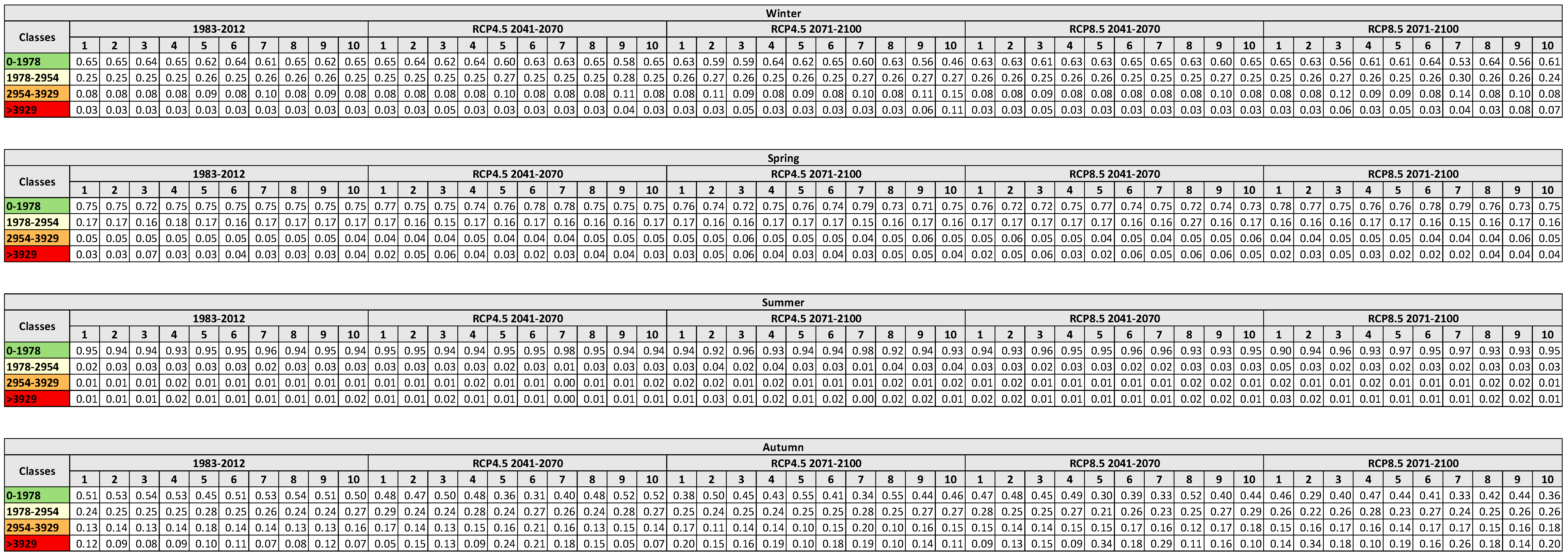
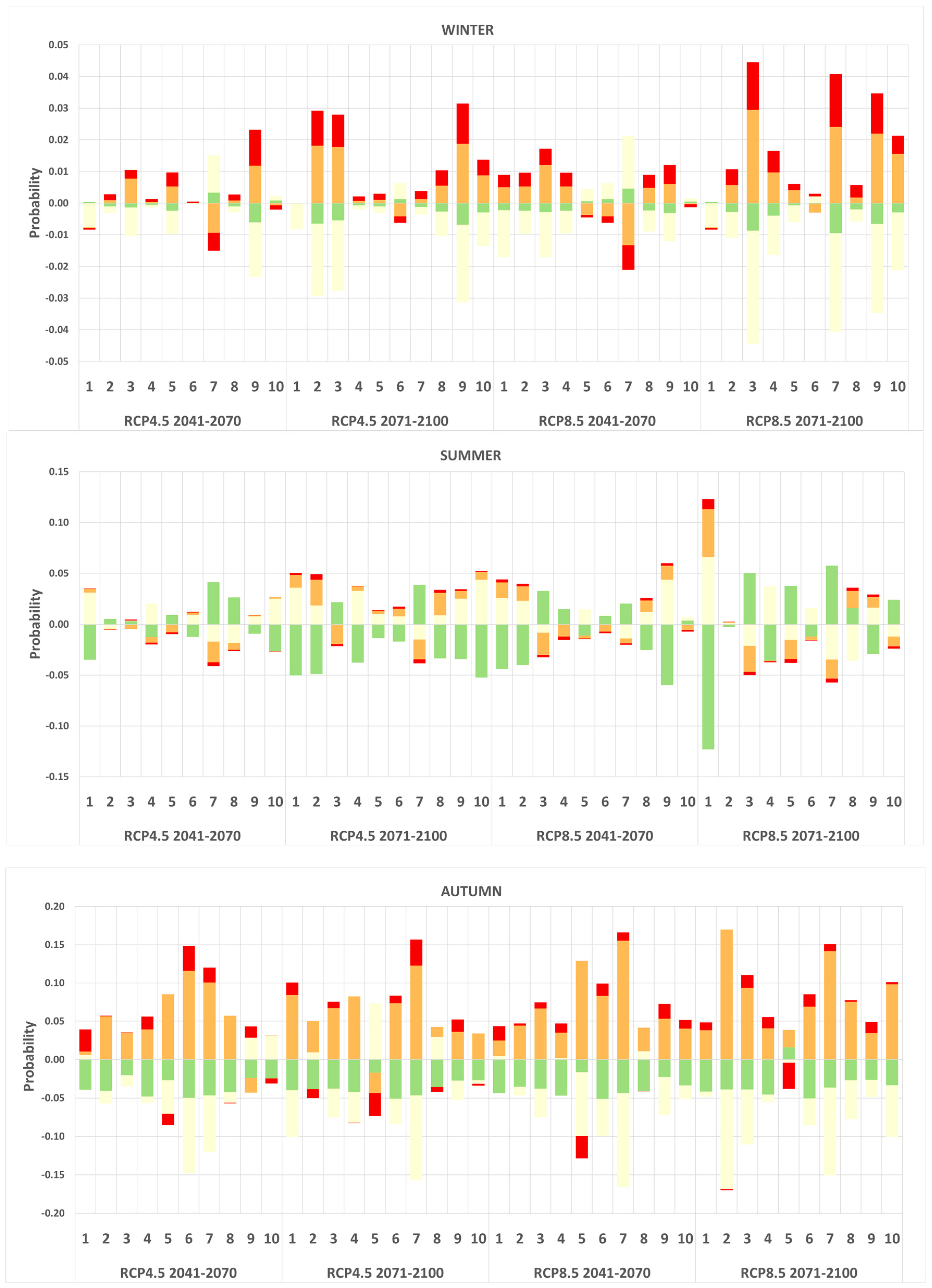
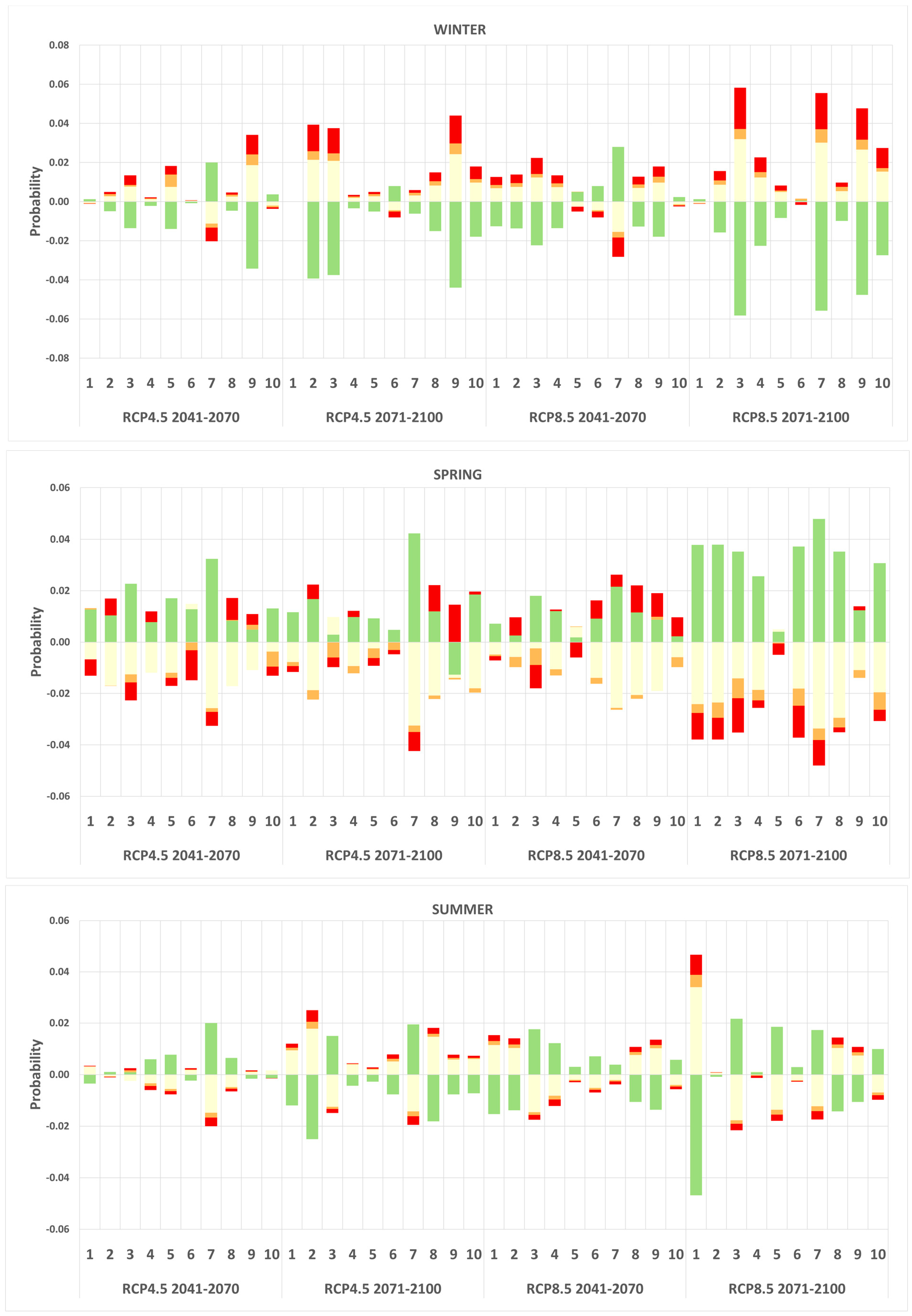
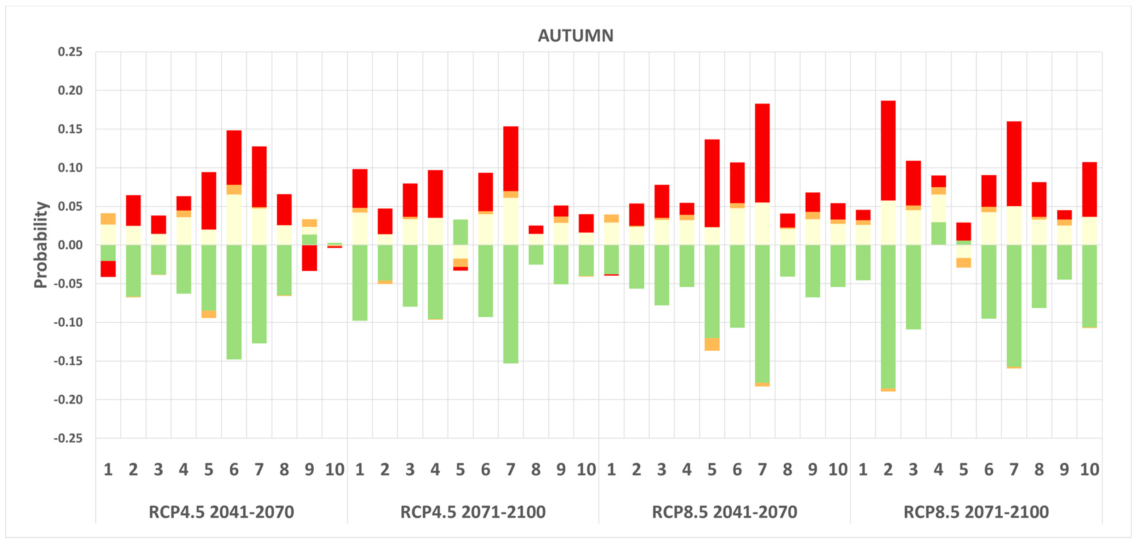
3.3. Hydrological Responses to Climate Change
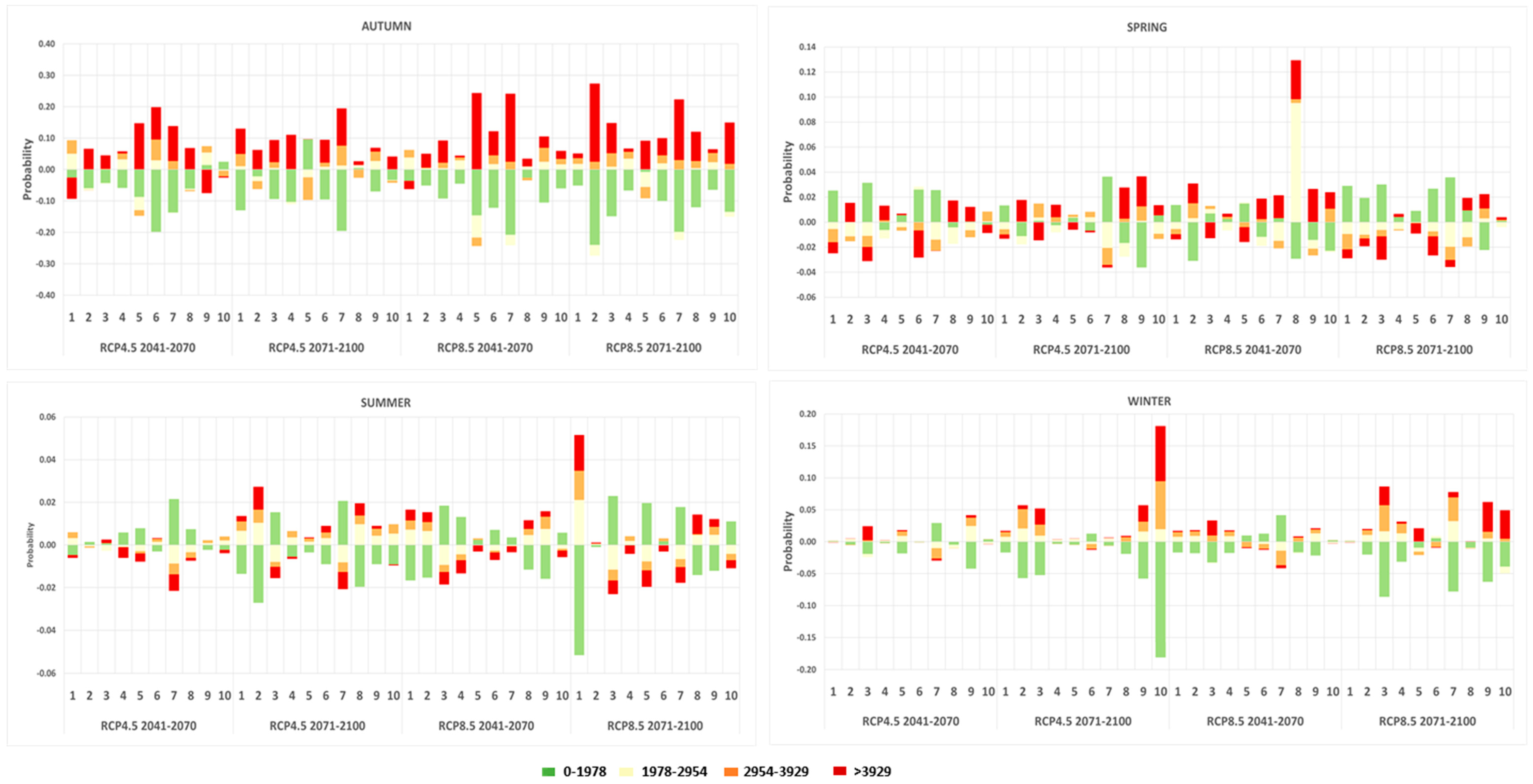
Uncertainty Analysis
4. Discussion and Conclusions
Author Contributions
Funding
Acknowledgments
Conflicts of Interest
Appendix

| Data Type | Description | Time Scale | Resolution | Source |
|---|---|---|---|---|
| Observations | ||||
| Land cover map |
| 2006 | 1:10,000 | Regione del Veneto Infrastruttura dati territoriali (http://idt.regione.veneto.it/app/metacatalog/) |
| Climatic data |
| 2004–2013 | 3 stations (i.e., Castelfranco, Veneto, Zero-Branco, Mogliano Veneto) (Figure 1) | ARPAV Servizio Meteorologico |
| Water quantity and quality data |
| 2007–2012 | 2 stations (i.e., manual station (Code 122), automatic station (Code: B2q) (Figure 1) | ARPAV Servizio Acque Interne MAV (Magistrato Acque Venezia) |
| Point-source pollution |
| 2004–2013 | 3 stations (i.e., Morgano, Zero-Branco, Castelfranco Veneto) (Figure 1) | ARPAV Servizio Acque Interne |
| Hydrological simulations | ||||
| Water quantity and quality data |
| 2004–2013 | River basin | SWAT (Soil Water Assessment Tool) simulations [30] |
| 2004–2013 | 1 station (i.e., manual station (Code 122) | ||
| Node | Description | Type | States | Parametrization Method |
|---|---|---|---|---|
| Season | Alternative seasons | Labeled | Winter | Expert judgement |
| Spring | ||||
| Summer | ||||
| Autumn | ||||
| Climate change scenario | Alternative climate change scenarios | Labeled | Baseline 1983–2012 | CMCC-CM/COSMO-CLM simulations |
| RCP 4.5 2041–2070 | ||||
| RCP 4.5 2071–2100 | ||||
| RCP 8.5 2041–2070 | ||||
| RCP 8.5 2071–2100 | ||||
| Agricultural land scenario | Extension of land (ha) occupied by agricultural activities under different scenarios | Labeled | Actual 2004–2013; | Observations, LUISA simulations |
| Future 2050 | ||||
| Temperature | Seasonal average temperature (°C) | Numeric interval | 0–8.37 | Observations |
| 8.37–13.79 | ||||
| 13.79–19.21 | ||||
| >19.21 | ||||
| Precipitation | Seasonal cumulative precipitation (mm) | Numeric interval | 0–201.50; | Observations |
| 201.50–328.73 | ||||
| 328.73–455.96 | ||||
| >455.96 | ||||
| Potential Evapotranspiration | Seasonal cumulative potential evapotranspiration (mm) | Numeric interval | 0–133.85 | Observations |
| 133.85–228.3 | ||||
| 228.3–322.75 | ||||
| >322.75 | ||||
| Effective rainfall | Seasonal cumulative effective rainfall reaching the soil (mm) | Numeric interval | 0–64.13 | SWAT simulations |
| 64.13–122.95 | ||||
| 122.95–181.77 | ||||
| >181.77 | ||||
| Crop water needs | Seasonal water demand for different crop typology (mm) | Numeric interval | 0–109.77 | Equation [36] |
| 109.77–213.64 | ||||
| 213.64–317.50 | ||||
| >317.50 | ||||
| Irrigation | Seasonal amount of water applied as irrigation | Numeric interval | <−55.29 | Equation [36] |
| −55.29–101.28 | ||||
| 101.28–257.86 | ||||
| >257.86 | ||||
| N fertilizer application | Nitrogen fertilizer applied for each season according to different crop typology (kg/ha) | Numeric interval | 0–45.74 | Expert judgment |
| 45.74–87.52 | ||||
| 87.52–129.30 | ||||
| >129.30 | ||||
| P fertilizer application | Phosphorus fertilizer applied for each season according to different crop typology (kg/ha) | Numeric interval | 0–25.41 | Expert judgment |
| 25.41–50.83 | ||||
| 50.83–76.25 | ||||
| >76.25 | ||||
| N diffuse sources | Seasonal amount of nitrogen coming from agricultural practices (kg) | Numeric interval | 0–7388.86 | Equation [36] |
| 7388.86–13,959.99 | ||||
| 13,959.99–20,531.11 | ||||
| >20,531.11 | ||||
| P diffuse sources | Seasonal amount of phosphorus coming from agricultural practices (kg) | Numeric interval | 0–5169.28 | Equation [36] |
| 5169.28–10,221.75 | ||||
| 10,221.75–15,274.21 | ||||
| >15,274.21 | ||||
| N point sources | Seasonal amount of nitrogen coming from point sources (i.e., wastewater treatment plants (WWTPs) and industrial discharges) (kg) | Numeric interval | 0–9382.64 | Observations |
| 9382.64–10,389.82 | ||||
| 10,389.82–11,396.99 | ||||
| >11,396.99 | ||||
| P point sources | Seasonal amount of phosphorus coming from point sources (i.e., WWTPs and industrial discharges) (kg) | Numeric interval | 0–1143.64 | Observations |
| 1143.64–1478.99 | ||||
| 1478.99–1814.35 | ||||
| >1814.35 | ||||
| River discharge | Seasonal average river discharge (L/s) | Numeric interval | 0–1458.96 | SWAT simulations |
| 1458.96–2360.53 | ||||
| 2360.535–3262.102 | ||||
| >3262.10 | ||||
| Runoff | Seasonal cumulative runoff (mm) | Numeric interval | 0–49.90 | SWAT simulations |
| 49.90–90.15 | ||||
| 90.15–130.40 | ||||
| >130.40 | ||||
| N in runoff | Seasonal amount of nitrogen loaded in the runoff (kg/ha) | Numeric interval | 0–0.63 | SWAT simulations |
| 0.63–1.19 | ||||
| 1.19–1.75 | ||||
| >1.75 | ||||
| P in runoff | Seasonal amount of phosphorus loaded in the runoff (kg/ha) | Numeric interval | 0–0.44 | SWAT simulations |
| 0.44–0.87 | ||||
| 0.87–1.30 | ||||
| >1.30 | ||||
| Total N loading | Seasonal nitrogen load in the river (kg) | Numeric interval | 0–17,031.20 | Equation [36] |
| 17,031.20–24,401.92 | ||||
| 24,401.92–31,772.64 | ||||
| > 31,772.64 | ||||
| Total P loading | Seasonal phosphorus load in the river (kg) | Numeric interval | 0–5405.76 | Equation [36] |
| 5405.76–9710.91 | ||||
| 9710.91–14,016.07 | ||||
| >14,016.07 | ||||
| Loading NO3− lagoon | Seasonal loading of NO3− reaching the lagoon (kg) | Numeric interval | 0–28,047.50 | SWAT simulations |
| 28,047.50–48,615.00 | ||||
| 48,615.00–69,182.50 | ||||
| >69,182.50 | ||||
| Loading NH4+ lagoon | Seasonal loading of NH4+ reaching the lagoon (kg) | Numeric interval | 0–3224.52 | SWAT simulations |
| 3224.52–5009.3 | ||||
| 5009.3–6794.17 | ||||
| >6794.17 | ||||
| Loading PO43− lagoon (kg) | Seasonal loading of PO43− reaching the lagoon (kg) | Numeric interval | 0–1978.90 | SWAT simulations |
| 1978.90–2954.00 | ||||
| 2954.00–3929.10 | ||||
| >3929.10 |


References
- Resolution, A. RES/70/1. Transforming our World: The 2030 Agenda for Sustainable Development. Available online: https://sustainabledevelopment.un.org/post2015/transformingourworld (accessed on 31 August 2019).
- Pasini, S.; Torresan, S.; Rizzi, J.; Zabeo, A.; Critto, A.; Marcomini, A. Climate change impact assessment in Veneto and Friuli Plain groundwater. Part II: a spatially resolved regional risk assessment. Sci. Total Environ. 2012, 440, 219–235. [Google Scholar] [CrossRef] [PubMed]
- Iyalomhe, F.; Rizzi, J.; Pasini, S.; Torresan, S.; Critto, A.; Marcomini, A. Regional Risk Assessment for climate change impacts on coastal aquifers. Sci. Total Environ. 2015, 537, 100–114. [Google Scholar] [CrossRef] [PubMed]
- Bussi, G.; Whitehead, P.G.; Bowes, M.J.; Read, D.S.; Prudhomme, C.; Dadson, S.J. Impacts of climate change, land-use change and phosphorus reduction on phytoplankton in the River Thames (UK). Sci. Total Environ. 2016, 572, 1507–1519. [Google Scholar] [CrossRef] [PubMed] [Green Version]
- Huttunen, I.; Lehtonen, H.; Huttunen, M.; Piirainen, V.; Korppoo, M.; Veijalainen, N.; Viitasalo, M.; Vehviläinen, B. Effects of climate change and agricultural adaptation on nutrient loading from Finnish catchments to the Baltic Sea. Sci. Total Environ. 2015, 529, 168–181. [Google Scholar] [CrossRef] [PubMed]
- Whitehead, P.; Butterfield, D.; Wade, D. Potential Impacts of Climate Change on River Water Quality; Environment Agency: Bristol, UK, 2008; ISBN 9781844329069. [Google Scholar]
- Carrasco, G.; Molina, J.-L.; Patino-Alonso, M.-C.; Castillo, M.D.C.; Vicente-Galindo, M.-P.; Galindo-Villardón, M.-P. Water quality evaluation through a multivariate statistical HJ-Biplot approach. J. Hydrol. 2019, 123993. [Google Scholar] [CrossRef]
- Molina, J.-L.; Zazo, S.; Martín, A.-M. Causal Reasoning: Towards Dynamic Predictive Models for Runoff Temporal Behavior of High Dependence Rivers. Water 2019, 11, 877. [Google Scholar] [CrossRef]
- Beck, M.; Krueger, T. The epistemic, ethical, and political dimensions of uncertainty in integrated assessment modeling. Wiley Interdiscip. Rev. Clim. Chang. 2016, 7, 627–645. [Google Scholar] [CrossRef]
- Carter, T.R.; Kenkyū, K.K.K.C.K. IPCC Technical Guidelines for Assessing Climate Change Impacts and Adaptations: Part of the IPCC Special Report to the First Session of the Conference of the Parties to the UN Framework Convention on Climate Change; IPCC: Geneva, Switzerland, 1994. [Google Scholar]
- Kundzewicz, Z.W.; Krysanova, V.; Benestad, R.E.; Hov, Ø.; Piniewski, M.; Otto, I.M. Uncertainty in climate change impacts on water resources. Environ. Sci. Policy 2018, 79, 1–8. [Google Scholar] [CrossRef]
- Parker, W.S. Ensemble modeling, uncertainty and robust predictions. Wiley Interdiscip. Rev. Clim. Chang. 2013, 4, 213–223. [Google Scholar] [CrossRef]
- Hawkins, E.; Sutton, R. The potential to narrow uncertainty in regional climate predictions. Bull. Am. Meteorol. Soc. 2009, 90, 1095–1108. [Google Scholar] [CrossRef]
- Ajami, N.K.; Hornberger, G.M.; Sunding, D.L. Sustainable water resource management under hydrological uncertainty. Water Resour. Res. 2008, 44. [Google Scholar] [CrossRef] [Green Version]
- Larson, K.; White, D.; Gober, P.; Wutich, A. Decision-making under uncertainty for water sustainability and urban climate change adaptation. Sustainability 2015, 7, 14761–14784. [Google Scholar] [CrossRef]
- Burgman, M. Risks and Decisions for Conservation and Environmental Management; Cambridge University Press: Cambridge, UK, 2005; ISBN 0521543010. [Google Scholar]
- Power, M.; McCarty, L.S. Environmental risk management decision-making in a societal context. Hum. Ecol. Risk Assess. 2006, 12, 18–27. [Google Scholar] [CrossRef]
- Uusitalo, L. Advantages and challenges of Bayesian networks in environmental modelling. Ecol. Model. 2007, 203, 312–318. [Google Scholar] [CrossRef]
- Wallach, D.; Mearns, L.O.; Ruane, A.C.; Rötter, R.P.; Asseng, S. Lessons from climate modeling on the design and use of ensembles for crop modeling. Clim. Chang. 2016, 139, 551–564. [Google Scholar] [CrossRef]
- IPCC. Climate Change 2007: Impacts, Adaptation and Vulnerability: Contribution of Working Group II to the Fourth Assessment Report of the Intergovernmental Panel on Climate Change (Parry M.L., Canziani O.F., Palutikof J.P., van der Linden P.J. e Hanson C.E.); Cambridge University Press: Cambridge, UK, 2007; ISBN 0521880106. [Google Scholar]
- Tebaldi, C.; Knutti, R. The use of the multi-model ensemble in probabilistic climate projections. Philos. Trans. R. Soc. Lond. A Math. Phys. Eng. Sci. 2007, 365, 2053–2075. [Google Scholar] [CrossRef] [PubMed]
- Martre, P.; Wallach, D.; Asseng, S.; Ewert, F.; Jones, J.W.; Rötter, R.P.; Boote, K.J.; Ruane, A.C.; Thorburn, P.J.; Cammarano, D. Multimodel ensembles of wheat growth: many models are better than one. Glob. Chang. Biol. 2015, 21, 911–925. [Google Scholar] [CrossRef]
- Krishnamurti, T.N.; Kishtawal, C.M.; Zhang, Z.; LaRow, T.; Bachiochi, D.; Williford, E.; Gadgil, S.; Surendran, S. Multimodel ensemble forecasts for weather and seasonal climate. J. Clim. 2000, 13, 4196–4216. [Google Scholar] [CrossRef]
- Luo, M.; Meng, F.; Liu, T.; Duan, Y.; Frankl, A.; Kurban, A.; De Maeyer, P. Multi–Model Ensemble Approaches to Assessment of Effects of Local Climate Change on Water Resources of the Hotan River Basin in Xinjiang, China. Water 2017, 9, 584. [Google Scholar] [CrossRef]
- Schellekens, J.; Dutra, E.; Martínez-de la Torre, A.; Balsamo, G.; van Dijk, A.; Weiland, F.S.; Minvielle, M.; Calvet, J.-C.; Decharme, B.; Eisner, S. A global water resources ensemble of hydrological models: The eartH2Observe Tier-1 dataset. Earth Syst. Sci. Data 2017, 9, 389. [Google Scholar] [CrossRef]
- Xu, H.; Brown, D.G.; Steiner, A.L. Sensitivity to climate change of land use and management patterns optimized for efficient mitigation of nutrient pollution. Clim. Chang. 2018, 147, 647–662. [Google Scholar] [CrossRef]
- Zuliani, A.; Zaggia, L.; Collavini, F.; Zonta, R. Freshwater discharge from the drainage basin to the Venice Lagoon (Italy). Environ. Int. 2005, 31, 929–938. [Google Scholar] [CrossRef] [PubMed]
- Osservatorio naturalistico della Laguna del Comune di Venezia; Guerzoni, S. Atlante Della Laguna: Venezia tra Terra e Mare; Marsilio: Venice, Italy, 2006; ISBN 8831787640. [Google Scholar]
- Facca, C.; Ceoldo, S.; Pellegrino, N.; Sfriso, A. Natural recovery and planned intervention in coastal wetlands: Venice Lagoon (Northern Adriatic Sea, Italy) as a case study. Sci. World J. 2014, 2014. [Google Scholar] [CrossRef] [PubMed]
- Pesce, M.; Critto, A.; Torresan, S.; Giubilato, E.; Santini, M.; Zirino, A.; Ouyang, W.; Marcomini, A. Modelling climate change impacts on nutrients and primary production in coastal waters. Sci. Total Environ. 2018, 628, 919–937. [Google Scholar] [CrossRef] [PubMed]
- Jacob, D.; Petersen, J.; Eggert, B.; Alias, A.; Christensen, O.B.; Bouwer, L.M.; Braun, A.; Colette, A.; Déqué, M.; Georgievski, G. EURO-CORDEX: new high-resolution climate change projections for European impact research. Reg. Environ. Chang. 2014, 14, 563–578. [Google Scholar] [CrossRef]
- Scoccimarro, E.; Gualdi, S.; Bellucci, A.; Sanna, A.; Fogli, P.G.; Manzini, E.; Vichi, M.; Oddo, P.; Navarra, A. Effects of Tropical Cyclones on Ocean Heat Transport in a High-Resolution Coupled General Circulation Model. J. Clim. 2011, 24, 4368–4384. [Google Scholar] [CrossRef] [Green Version]
- Cattaneo, L.; Zollo, A.L.; Bucchignani, E.; Montesarchio, M.; Manzi, M.P.; Mercogliano, P. Assessment of Cosmo-Clm Performances over Mediterranean Area. SSRN Electron. J. 2012. [Google Scholar] [CrossRef]
- Thomson, A.M.; Calvin, K.V.; Smith, S.J.; Kyle, G.P.; Volke, A.; Patel, P.; Delgado-Arias, S.; Bond-Lamberty, B.; Wise, M.A.; Clarke, L.E. RCP 4.5: A pathway for stabilization of radiative forcing by 2100. Clim. Chang. 2011, 109, 77. [Google Scholar] [CrossRef]
- Riahi, K.; Rao, S.; Krey, V.; Cho, C.; Chirkov, V.; Fischer, G. RCP 8.5—A scenario of comparatively high greenhouse gas emissions. Clim. Chang. 2011, 109, 33–57. [Google Scholar] [CrossRef]
- Sperotto, A.; Molina, J.L.; Torresan, S.; Critto, A.; Pulido-Velazquez, M.; Marcomini, A. A Bayesian Networks approach for the assessment of climate change impacts on nutrients loading. Environ. Sci. Policy 2019, 100, 21–36. [Google Scholar] [CrossRef]
- Madsen, A.L.; Jensen, F.; Kjaerulff, U.B.; Lang, M. The Hugin tool for probabilistic graphical models. Int. J. Artif. Intell. Tools 2005, 14, 507–543. [Google Scholar] [CrossRef]
- Bromley, J.; Jackson, N.A.; Clymer, O.J.; Giacomello, A.M.; Jensen, F.V. The use of Hugin® to develop Bayesian networks as an aid to integrated water resource planning. Environ. Model. Softw. 2005, 20, 231–242. [Google Scholar] [CrossRef]
- Arnold, J.G.; Moriasi, D.N.; Gassman, P.W.; Abbaspour, K.C.; White, M.J.; Srinivasan, R.; Santhi, C.; Harmel, R.D.; Van Griensven, A.; Van Liew, M.W. SWAT: Model use, calibration, and validation. Trans. ASABE 2012, 55, 1491–1508. [Google Scholar] [CrossRef]
- Marcot, B.G. Metrics for evaluating performance and uncertainty of Bayesian network models. Ecol. Model. 2012, 230, 50–62. [Google Scholar] [CrossRef]
- Kragt, M.E. A Beginners Guide to Bayesian Network Modelling for Integrated Catchment Management. Available online: http://www.landscapelogic.org.au/publications/Technical_Reports/No_9_BNs_for_Integrated_Catchment_Management.pdf (accessed on 30 August 2019).
- Molina, J.-L.; Zazo, S.; Rodríguez-Gonzálvez, P.; González-Aguilera, D. Innovative Analysis of Runoff Temporal Behavior through Bayesian Networks. Water 2016, 8, 484. [Google Scholar] [CrossRef]
- Pearl, J. Probabilistic Reasoning in Intelligent Systems: Networks of Plausible Inference; Morgan Kaufmann: Burlington, MA, USA, 1988; ISBN 0080514898. [Google Scholar]
- Pollino, C.A.; Woodberry, O.; Nicholson, A.; Korb, K.; Hart, B.T. Parameterisation and evaluation of a Bayesian network for use in an ecological risk assessment. Environ. Model. Softw. 2007, 22, 1140–1152. [Google Scholar] [CrossRef]
- Pesce, M.; Critto, A.; Torresan, S.; Giubilato, E.; Pizzol, L.; Marcomini, A. Assessing uncertainty of hydrological and ecological parameters originating from the application of an ensemble of ten global-regional climate model projections in a coastal ecosystem of the lagoon of Venice, Italy. Ecol. Eng. 2019, 133, 121–136. [Google Scholar] [CrossRef]
- Bouraoui, F.; Galbiati, L.; Bidoglio, G. Climate change impacts on nutrient loads in the Yorkshire Ouse catchment (UK). Hydrol. Earth Syst. Sci. Discuss. 2002, 6, 197–209. [Google Scholar] [CrossRef]
- Panagopoulos, Y.; Makropoulos, C.; Mimikou, M. Diffuse surface water pollution: Driving factors for different geoclimatic regions. Water Resour. Manag. 2011, 25, 3635. [Google Scholar] [CrossRef]
- Molina, J.-L.; Pulido-Velázquez, D.; García-Aróstegui, J.L.; Pulido-Velázquez, M. Dynamic Bayesian networks as a decision support tool for assessing climate change impacts on highly stressed groundwater systems. J. Hydrol. 2013, 479, 113–129. [Google Scholar] [CrossRef]


| No. | Global Climate Model (GCM) | Regional Climate Model (RCM) | Representative Concentration Pathways (RCPs) | Resolution | Time Range | Institute |
|---|---|---|---|---|---|---|
| 1 | HadGEM2-ES | RCA4 | 4.5, 8.5 | 12 km | 1970–2099 | SMHI |
| 2 | IPSL-CM5A-MR | RCA5 | 4.5, 8.6 | 12 km | 1970–2100 | SMHI |
| 3 | CNRM-CM5 | RCA6 | 4.5, 8.7 | 12 km | 1970–2100 | SMHI |
| 4 | EC-EARTH | RCA7 | 4.5, 8.8 | 12 km | 1970–2100 | SMHI |
| 5 | MPI-ESM-LR | RCA8 | 4.5, 8.9 | 12 km | 1970–2100 | SMHI |
| 6 | CNRM-CM5 | CCLM | 4.5, 8.10 | 12 km | 1950–2100 | CLMcom |
| 7 | CMCC-CM | COSMO-CLM | 4.5, 8.11 | 8 km | 1976–2100 | CMCC |
| 8 | HadGEM2-ES | RACMO22E | 4.5, 8.12 | 12 km | 1950–2099 | KNMI |
| 9 | EC-EARTH | HIRHAM5 | 4.5, 8.13 | 12 km | 1951–2100 | DMI |
| 10 | EC-EARTH | RACMO22E | 4.5, 8.14 | 12 km | 1950–2100 | KNMI |
| Variable | Entropy H(x) |
|---|---|
| Effective rainfall | 3.26 |
| Season | 1.39 |
| Temperature | 1.38 |
| N point sources | 1.36 |
| River flow | 1.34 |
| N runoff | 1.33 |
| N diffuse sources | 1.33 |
| Total N Loading | 1.31 |
| Evapotranspiration | 1.28 |
| Loading NO3− | 1.24 |
| Irrigation | 1.24 |
| P point sources | 1.17 |
| Runoff | 1.12 |
| Precipitation | 1.06 |
| N fertilizer application | 1.04 |
| Loading NH4+ | 0.98 |
| Loading PO43− | 0.97 |
| P runoff | 0.96 |
| P diffuse sources | 0.96 |
| Water needs | 0.56 |
| P fertilizer application | 0.56 |
| Sensitive Node | Node Affecting Sensitivity | MI |
|---|---|---|
| Loading NO3− | River flow | 0.54 |
| Total N loading | 0.30 | |
| N diffuse sources | 0.23 | |
| N runoff | 0.23 | |
| Evapotranspiration | 0.23 | |
| Loading NH4+ | River flow | 0.37 |
| Loading NO3− | 0.18 | |
| Total N loading | 0.17 | |
| Runoff | 0.15 | |
| N diffuse sources | 0.11 | |
| Loading PO43− | Total P loading | 0.53 |
| P runoff | 0.39 | |
| P diffuse sources | 0.39 | |
| River flow | 0.34 | |
| Runoff | 0.31 |
© 2019 by the authors. Licensee MDPI, Basel, Switzerland. This article is an open access article distributed under the terms and conditions of the Creative Commons Attribution (CC BY) license (http://creativecommons.org/licenses/by/4.0/).
Share and Cite
Sperotto, A.; Molina, J.L.; Torresan, S.; Critto, A.; Pulido-Velazquez, M.; Marcomini, A. Water Quality Sustainability Evaluation under Uncertainty: A Multi-Scenario Analysis Based on Bayesian Networks. Sustainability 2019, 11, 4764. https://doi.org/10.3390/su11174764
Sperotto A, Molina JL, Torresan S, Critto A, Pulido-Velazquez M, Marcomini A. Water Quality Sustainability Evaluation under Uncertainty: A Multi-Scenario Analysis Based on Bayesian Networks. Sustainability. 2019; 11(17):4764. https://doi.org/10.3390/su11174764
Chicago/Turabian StyleSperotto, Anna, Josè Luis Molina, Silvia Torresan, Andrea Critto, Manuel Pulido-Velazquez, and Antonio Marcomini. 2019. "Water Quality Sustainability Evaluation under Uncertainty: A Multi-Scenario Analysis Based on Bayesian Networks" Sustainability 11, no. 17: 4764. https://doi.org/10.3390/su11174764