1. Introduction
The water footprint and related concepts, like the ecological footprint (Costanza [
1]) or the carbon footprint (Weber and Matthews [
2]), are aimed at gauging the impact of economic activities on natural resources. In particular, the water footprint is increasingly being used as an indicator of the human pressure on water resources (Hoekstra and Mekonnen [
3]), and efforts are under way to set standard rules for its process of construction (Hoekstra
et al. [
4]).
The water footprint is an intrinsically static notion, since it measures the amount of water usage in a specific time period. However, a series of water footprints could be computed for a number of consecutive periods. The availability of a time series of footprints would allow one to assess how such a “footpath” evolves over time, what forces are driving its temporal evolution and, as it is possible to distinguish among several types of water consumption, the dynamics of its various internal components.
The construction of a water footpath is made difficult by demanding data requirements. To the best of our knowledge, only Cazcarro, Duarte and Sánchez-Chóliz [
5] have estimated and analyzed a water footprint time series (for Spain), whereas Wiedmann
et al. [
6] undertook a similar investigation for the carbon footprint in the U.K. These are single country studies, and comparative analyses of different footpaths among different countries have not been realized as yet.
This paper is precisely about the construction, decomposition and comparison of water footprint time series in 40 countries and one aggregate macro-region, in the period 1995–2009. The estimation of water footpaths is made possible by the availability of time series for multi-regional input-output tables, realized by the World Input-Output Database (WIOD) project (Dietzenbacher
et al. [
7]).
The next section illustrates how water footprints can be computed from a database of input-output trade flows, like the WIOD.
Section 3 further discusses how the inter-annual variations of footprints have been decomposed in this study. We compute production and consumption footprints, which are those related to production activities (using water resources in the country where production is carried out) and to consumption levels (requiring water from different regions through imported commodities). In both cases, we break down the changes as variations in: (1) the aggregate activity level (total gross production, total consumption); (2) the industrial composition; and (3) the water efficiency or productivity. Furthermore, we separately compute production footpaths for blue, green and grey water. For consumption footpaths, we separate footprints for intermediate and final consumption (we disregard water footprints stemming from investment demand, as this is highly volatile and often negative, due to changes in inventories).
The analysis and comparison of the different footpaths, which is presented in the fourth section of this paper, allows us to speculate about the causes behind the time evolution of water footprints in the various countries. This analysis provides some general insights, which are useful for a better understanding of how the pressure on water resources may change in the future.
A concluding section summarizes and lays out some final comments.
3. Data and Methodology
The WIOD project provides complete multi-regional input-output tables for the years 1995–2009, including all 27 countries in the European Union, 17 other countries and one remaining “Rest of the World” aggregate region. Each annual table gives information about production levels (in U.S. dollars) for 35 industries in every region, as well as intermediate industrial consumption (for all industries), public and private consumption, investments and inventory changes. All consumption items are expressed as vectors, in which both the industrial and the regional origins of trade flows are specified.
The input-output tables, which are estimated on the basis of official national accounts (Dietzenbacher
et al. [
7]), are accompanied by “satellite environmental accounts”, expressed in physical units of measure (Genty, Arto and Neuwahl [
11]). The variables covered are: use of energy; emission of main greenhouse gases; emission of other main air pollutants; use of mineral and fossil resources; land and water use. For water, estimates are obtained through elaboration from original data by Mekonnen and Hoekstra [
9,
12,
13,
14] and separately consider blue, green and grey water.
All water footprints are scalar numbers (f), obtainable through multiplication of a row vector w of water coefficients (water usage per unit) by a column vector a of economic activity levels:
In our setting,
w includes ratios of water industrial consumption over output value (1000 cubic meters per dollar). When estimating production footprints, in a given year and country, the
w vector includes 35 elements (one for each industry), and the
a vector corresponds to the vector of industrial output. In the case of consumption footprint, the
w vector includes 35 × 41 elements (industry by country), and the
a vector is the sum over all 35 + 5 consumption vectors (This is because, in all countries, there are 35 industries generating demand for intermediate inputs (whose production may require water), plus one household sector, one private non-profit organizations sector, one public sector, investments in physical capital formation and changes in inventory stocks (5 final demand sectors); notice that intermediate consumption is included. The 35 + 5 vectors correspond to the light blue columns in
Figure 1 and to the R + CR columns in
Appendix A.).
The same formula is applicable for the computation of components of total water footprints. For example, to get the blue water footprint, it is sufficient to consider only blue water in the vector w. Analogously, to get the footprint due to final consumption, only the latter component of demand should be inserted into the vector a.
The change of a water footprint from one year t to the following year t + 1 can be traced back to variations in the elements of vectors w and a. To single out the effects of aggregate growth, a factor g can be computed, such that the new total is obtained by proportionally scaling all elements:
This allows us to decompose the variation in the footprint indicator in three steps:
The first step, corresponding to the first element of the sum in the right-hand side of Equation (3), is readily interpreted as the change in water footprint induced by the change in aggregate activity (total production or consumption levels). The second step can be interpreted as the contribution due to variations in the structure of the a vector (production or consumption patterns). Finally, the last element refers to variations in the elements of the w vector, expressing the coefficients of water productivity.
In this work, we estimated water footprints for production and consumption for 41 regions and 15 years, from 1995–2009. In all series, we consider the percentage variation (more precisely, the difference in logarithms) of the water footprint from the previous year, and we decompose this change into the three elements of activity level, activity pattern and water efficiency. We also produce production footprint time series for blue, green and grey water, as well as separate footprints for intermediate and final consumption. The results are presented and discussed in the following section.
4. Results
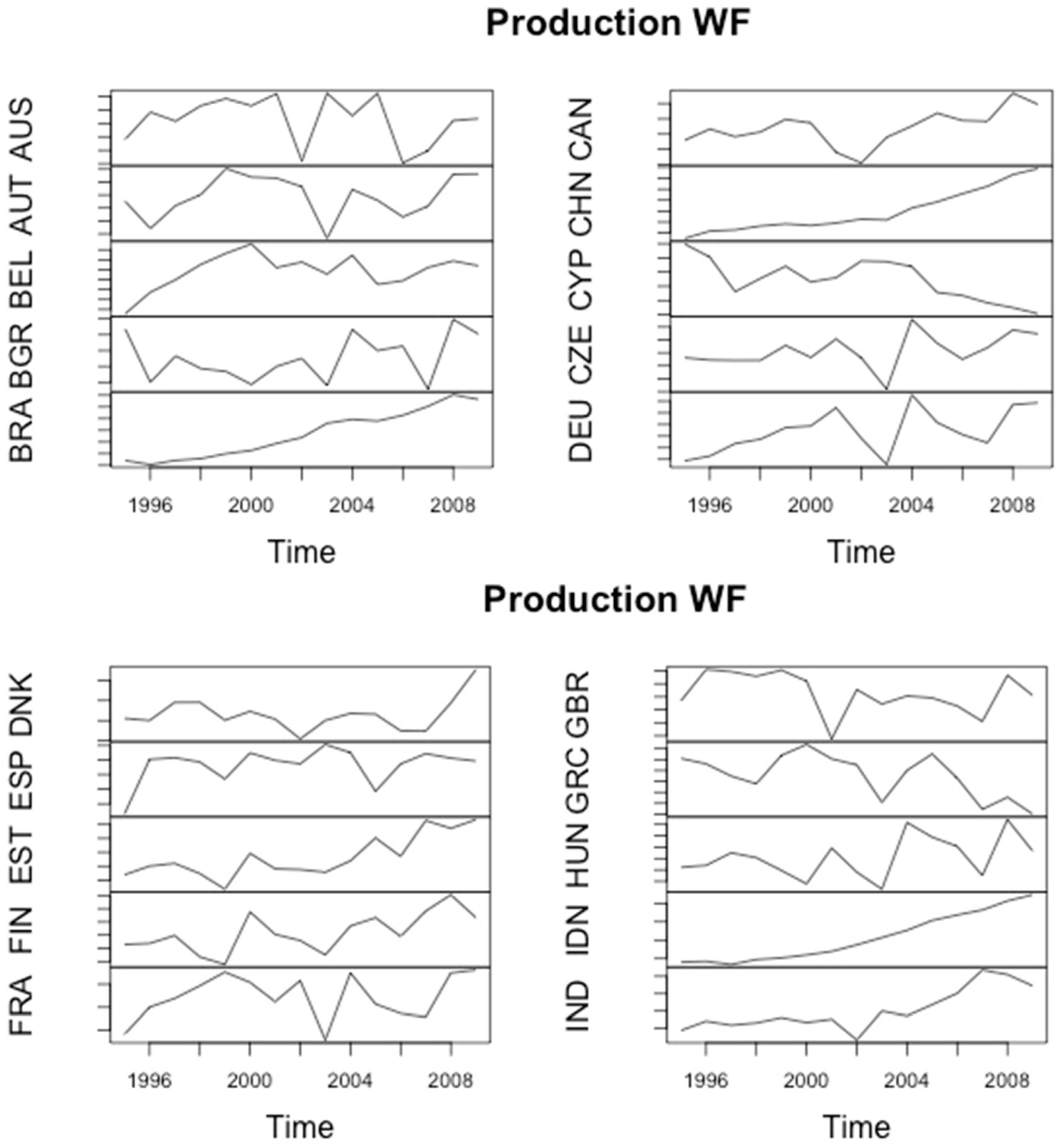
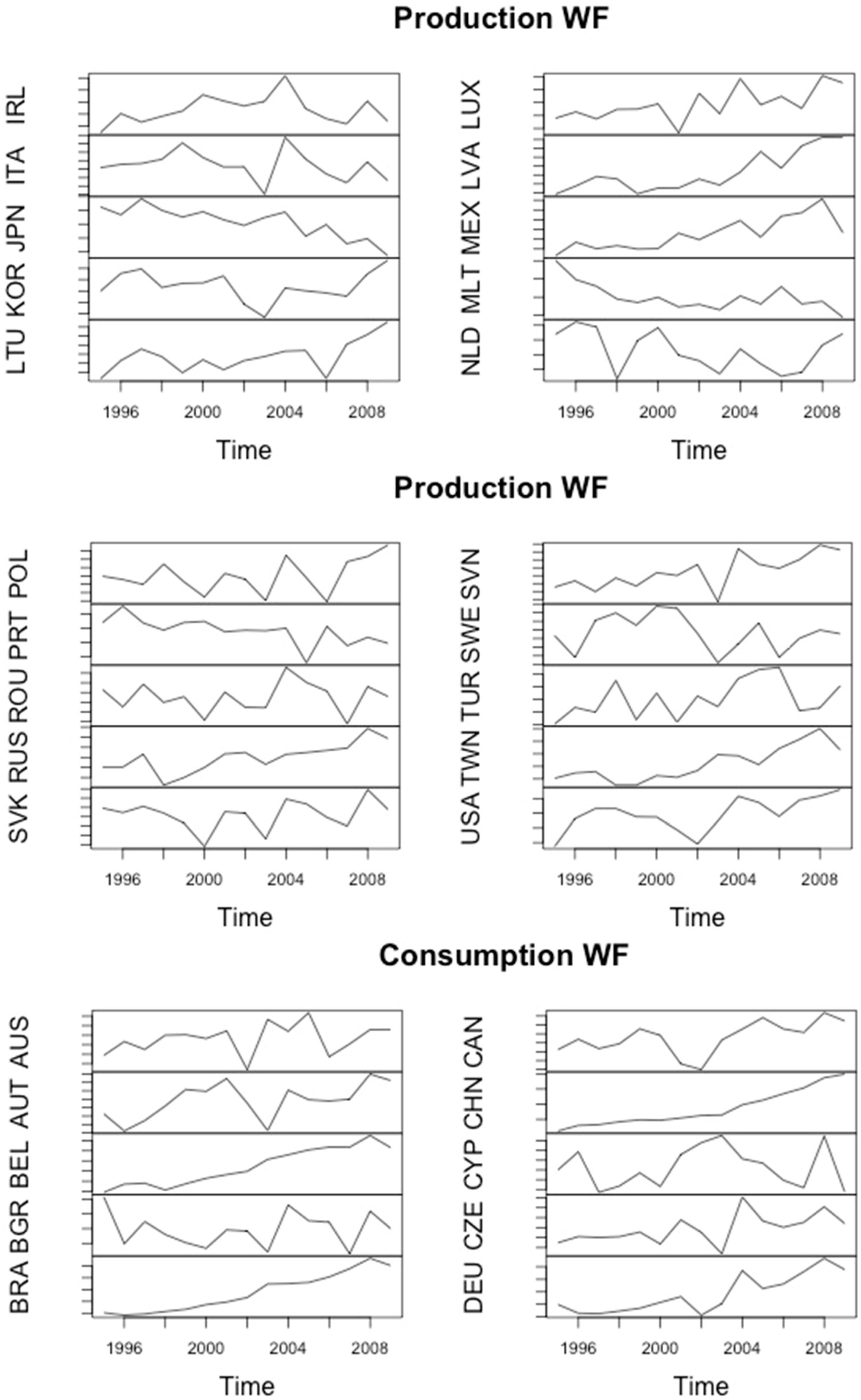
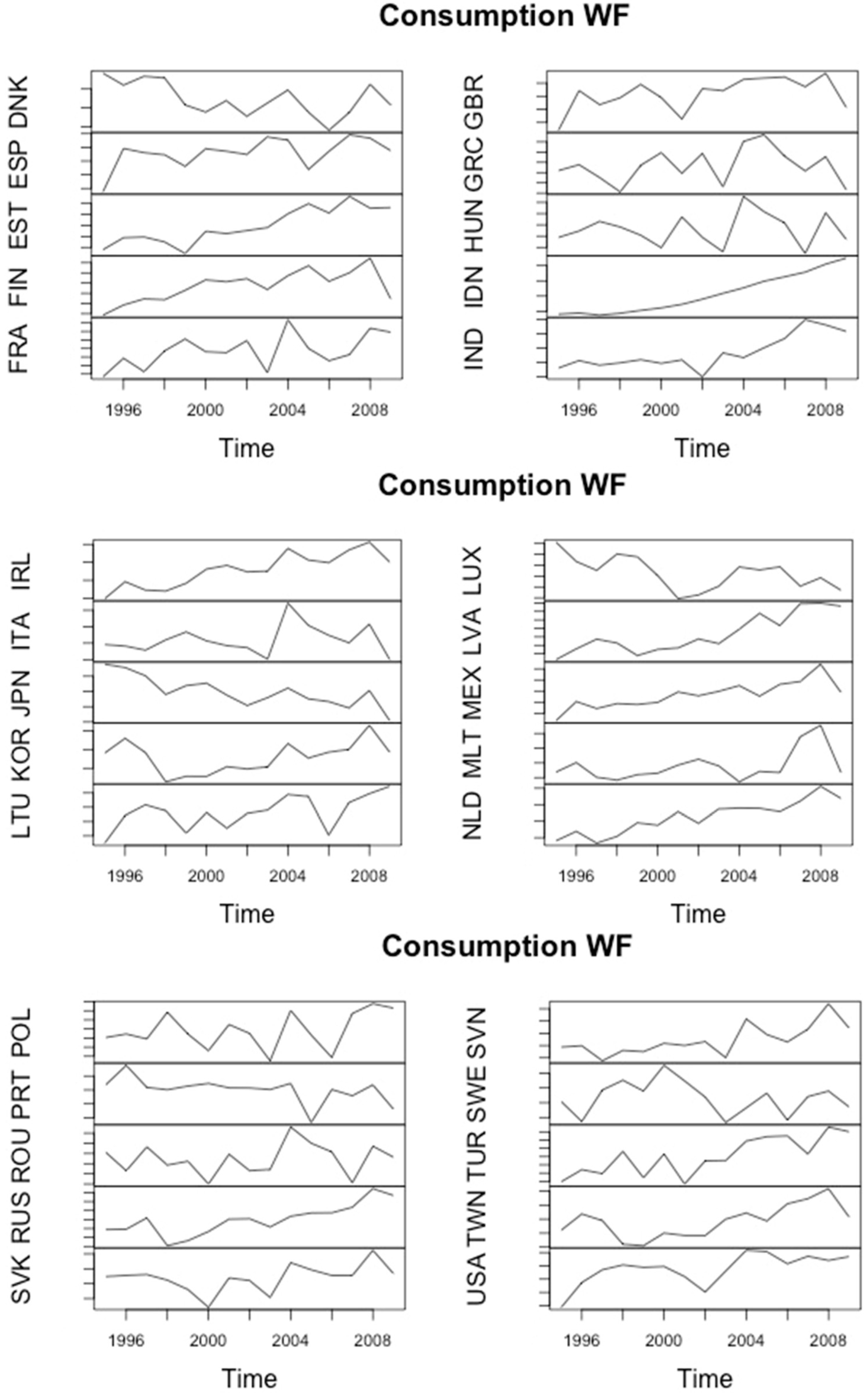
Series of stacked graphs, displaying “footpaths” for individual countries, both for production and consumption, are displayed in
Appendix B (
Figure A1). In most cases, it is difficult to devise a clear trend, except for the BRIC countries of Brazil, India, China and Russia, with the addition of Indonesia, where economic growth was strongest and where water footprints are characterized by a steady increase over time. The influence of economic growth is also evident through the impact of temporary economic crises, like that of 1998 in Russia. The global economic slowdown of 2009 can also be seen in many countries, in terms of the reduction or stabilization of water footprints in the last year.
Table 1 reports some summary statistics about the water footprint time series for production. Average annual growth rates are displayed in the second column. We can see that most countries exhibit positive, but not very large increments, whereas some other countries reduce their footprint. The largest increases, above 3% of the average annual growth rate, are found in Brazil, China, Spain, Estonia, Indonesia, Lithuania and Latvia. These are all countries that have experienced sustained growth in the period 1995–2009 and an expansion of production in agricultural sectors. Bulgaria, Cyprus, Greece, Italy, Japan, Malta, Portugal, Romania and Slovakia have diminished their production footprint in the same period.
We decompose the average variation in three stages, according to Equation (3). The third column (Var. levels1) displays the average growth rate attributable to the aggregate increase in production levels. As expected, all rates are positive, with the exception of Japan, which has been affected by a prolonged recession.
One potential problem here is that the activity levels refer to nominal production values, not quantities. Therefore, an increase in the aggregate activity level is generally due to both real production and inflation. This explains why figures could be higher and more volatile than macroeconomic data.
As an alternative measure for the aggregate growth component, we compute the average annual variation using real GDP growth rates (World Bank, 2014) [
15] instead of the
g factor, as defined in Equation (2). Results, which are indeed more homogeneous and with lower figures, are shown in the fourth column (Var. levels2).
The next column (Var. struct.) gives the variation of the footprint induced by changes in the pattern of industrial production. Interestingly, all rates (with minor exceptions in Austria, Brazil and Indonesia) are negative and often quite significantly so. This means that the productive structure in most economies has shifted away from water-intensive industries, most notably agriculture. Furthermore, the correlation coefficient between average changes in levels and average changes in patterns is found to be −0.55, suggesting that high-growth countries are also countries in which the share of agriculture shrinks at a faster pace, possibly because of the expansion in manufacturing and services.
The last two columns display the remaining component attributable to water efficiency. Here, we have two values, corresponding to the two values of the changes in levels. A negative number should be interpreted as an improvement in water efficiency, which is in the value of production per unit of water. We can see that improvements in water productivity are typically found only when they are associated with high growth rates in aggregate production levels, whereas this result no longer holds true, in general, with more prudential growth rates.
Table 1.
Production WFs (yearly av. changes): decomposition.
Table 1.
Production WFs (yearly av. changes): decomposition.
| Country | WF av. var. | Var. levels1 | Var. levels2 | Var. struct. | Var. eff.1 | Var. eff.2 |
|---|
| Australia | 0.88% | 6.87% | 3.55% | −3.28% | −2.71% | 0.61% |
| Austria | 0.48% | 4.26% | 2.08% | 0.91% | −4.70% | −2.52% |
| Belgium | 0.58% | 3.87% | 1.86% | −3.26% | −0.03% | 1.98% |
| Bulgaria | −0.19% | 9.42% | 3.07% | −6.69% | −2.93% | 3.43% |
| Brazil | 3.16% | 5.54% | 2.79% | 0.62% | −3.00% | −0.25% |
| Canada | 1.32% | 6.05% | 2.57% | −2.38% | −2.35% | 1.12% |
| China | 3.39% | 14.87% | 10.01% | −4.40% | −7.08% | −2.22% |
| Cyprus | −4.24% | 7.16% | 3.32% | −5.21% | −6.19% | −2.36% |
| Czech Rep. | 0.91% | 8.89% | 2.94% | −5.30% | −2.69% | 3.26% |
| Germany | 1.18% | 2.29% | 1.09% | −1.29% | 0.18% | 1.38% |
| Denmark | 0.86% | 4.36% | 1.36% | −3.95% | 0.45% | 3.44% |
| Spain | 3.71% | 6.71% | 2.96% | −4.20% | 1.20% | 4.95% |
| Estonia | 3.95% | 10.74% | 4.93% | −5.58% | −1.22% | 4.60% |
| Finland | 0.75% | 4.80% | 2.77% | −2.29% | −1.76% | 0.27% |
| France | 0.99% | 3.91% | 1.65% | −2.59% | −0.33% | 1.92% |
| Great Britain | 0.10% | 4.60% | 2.41% | -4.52% | 0.03% | 2.22% |
| Greece | −1.05% | 5.93% | 3.08% | −5.62% | −1.36% | 1.48% |
| Hungary | 0.74% | 7.59% | 2.41% | −5.01% | −1.84% | 3.34% |
| Indonesia | 3.49% | 6.04% | 3.65% | 0.23% | −2.78% | −0.39% |
| India | 1.51% | 9.07% | 6.83% | −3.07% | −4.49% | −2.25% |
| Ireland | 0.30% | 9.11% | 5.56% | −11.45% | 2.64% | 6.19% |
| Italy | −0.30% | 4.62% | 0.84% | −2.25% | −2.67% | 1.11% |
| Japan | −0.99% | −0.36% | 0.54% | −0.48% | −0.15% | −1.05% |
| Korea | 0.53% | 4.52% | 4.62% | −4.19% | 0.20% | 0.10% |
| Lithuania | 4.45% | 11.35% | 4.81% | −6.64% | -0.26% | 6.28% |
| Luxembourg | 1.14% | 9.30% | 3.85% | −7.41% | −0.76% | 4.70% |
| Latvia | 4.26% | 12.31% | 4.96% | −5.14% | −2.91% | 4.45% |
| Mexico | 0.59% | 6.88% | 2.76% | −1.72% | −4.57% | −0.45% |
| Malta | −2.16% | 6.10% | 2.70% | −1.34% | −6.92% | −3.52% |
| The Netherlands | 0.01% | 4.71% | 2.31% | −2.86% | −1.84% | 0.56% |
| Poland | 0.87% | 8.46% | 4.46% | −5.33% | −2.27% | 1.73% |
| Portugal | −1.37% | 5.06% | 1.88% | −2.80% | −3.63% | −0.45% |
| Romania | −0.52% | 9.77% | 2.81% | −4.95% | −5.34% | 1.62% |
| Russia | 2.15% | 9.10% | 3.84% | −3.71% | −3.25% | 2.02% |
| Slovakia | −0.07% | 10.43% | 4.38% | −3.67% | −6.84% | −0.79% |
| Slovenia | 1.17% | 6.20% | 3.43% | −2.63% | −2.41% | 0.36% |
| Sweden | 0.06% | 3.53% | 2.36% | −0.55% | −2.92% | −1.75% |
| Turkey | 0.93% | 7.64% | 3.68% | −1.92% | −4.79% | −0.84% |
| Taiwan | 1.58% | 2.39% | 3.91% | −3.78% | 2.98% | 1.46% |
| United States | 1.28% | 4.36% | 2.55% | −1.67% | −1.41% | 0.39% |
| Rest of World | 2.63% | 6.88% | 3.29% | −0.82% | −3.43% | 0.16% |
Perhaps one may be surprised, and suspicious, about the finding that water productivity may have worsened in many countries, since improvements in cultivation and irrigation techniques should have improved efficiency. This reasoning is not readily applicable at the aggregate level, though, because we are not considering here production factors different from water, and the output is measured in monetary terms. For instance, higher water usage could partly compensate the lower productivity of other inputs, including non-market factors associated with climatic conditions. Water footprints are computed at the crop level on the basis of yield per hectare and climatic conditions. However, several crops are considered within the same agricultural industry. To see how factor substitution may work at the aggregate level, suppose that an industry includes two crops: the first one labor intensive, the second one water intensive. After a drop in labor productivity, the relative profitability of Crop 1 diminishes, and the production mix changes with more land allocated to Crop 2. For the industry as a whole, this implies more water per unit of output.
Table 2 provides results for a similar kind of exercise, this time applied to the series of consumption water footprints. The time profiles of footprints (
Appendix B), as well as average annual growth rates (second column in
Table 2) are quite similar to those of production footprints. Significant divergences can be found in small, open economies, like Belgium (average 3.53% for consumption
vs. 0.58% for production), because a large share of domestic consumption is imported, whereas differences are slight in large, relatively closed economies, like the United States (1.26%
vs. 1.28%), where most domestic consumption is covered by internal production.
Table 2.
Consumption WFs (yearly av. changes): decomposition.
Table 2.
Consumption WFs (yearly av. changes): decomposition.
| Country | WF av. var. | Var. levels1 | Var. levels2 | Var. struct. | Var. eff.1 | Var. eff.2 | |
|---|
| Australia | 1.91% | 7.37% | 3.55% | −2.75% | −2.72% | 1.11% | |
| Austria | 0.70% | 5.50% | 2.08% | −0.73% | −4.06% | −0.64% | |
| Belgium | 3.53% | 6.13% | 1.86% | −0.26% | −2.34% | 1.93% | |
| Bulgaria | −1.53% | 12.86% | 3.07% | −11.57% | −2.82% | 6.98% | |
| Brazil | 2.62% | 6.65% | 2.79% | −1.01% | −3.03% | 0.84% | |
| Canada | 1.01% | 7.75% | 2.57% | −4.31% | −2.43% | 2.75% | |
| China | 3.86% | 13.80% | 10.01% | −3.03% | −6.91% | −3.12% | |
| Cyprus | −0.74% | 9.77% | 3.32% | −5.96% | −4.55% | 1.90% | |
| Czech Rep. | 0.89% | 12.27% | 2.94% | −8.63% | −2.75% | 6.58% | |
| Germany | 0.85% | 4.04% | 1.09% | −1.91% | −1.28% | 1.68% | |
| Denmark | −0.48% | 6.95% | 1.36% | −6.90% | −0.53% | 5.05% | |
| Spain | 2.63% | 8.56% | 2.96% | −6.04% | 0.11% | 5.71% | |
| Estonia | 4.20% | 14.48% | 4.93% | −8.77% | −1.51% | 8.04% | |
| Finland | 0.90% | 8.44% | 2.77% | −5.33% | −2.21% | 3.46% | |
| France | 0.65% | 5.42% | 1.65% | −3.93% | −0.83% | 2.93% | |
| Great Britain | 0.47% | 7.78% | 2.41% | −6.00% | −1.31% | 4.05% | |
| Greece | −0.33% | 7.73% | 3.08% | −6.37% | −1.68% | 2.96% | |
| Hungary | −0.11% | 11.26% | 2.41% | −9.50% | −1.87% | 6.98% | |
| Indonesia | 3.51% | 4.70% | 3.65% | 1.67% | −2.87% | −1.81% | |
| India | 1.54% | 8.80% | 6.83% | −2.77% | −4.49% | −2.52% | |
| Ireland | 1.21% | 12.46% | 5.56% | −12.12% | 0.88% | 7.77% | |
| Italy | −0.34% | 7.12% | 0.84% | −4.72% | −2.74% | 3.55% | |
| Japan | −2.06% | 1.10% | 0.54% | −1.59% | −1.57% | −1.01% | |
| Korea | 0.03% | 7.11% | 4.62% | −5.06% | −2.01% | 0.47% | |
| Lithuania | 3.41% | 15.82% | 4.81% | −11.90% | −0.51% | 10.50% | |
| Luxembourg | −1.88% | 11.63% | 3.85% | −10.88% | −2.64% | 5.14% | |
| Latvia | 4.45% | 16.18% | 4.96% | −8.78% | −2.94% | 8.28% | |
| Mexico | 1.25% | 10.41% | 2.76% | −4.85% | −4.31% | 3.35% | |
| Malta | −0.05% | 10.47% | 2.70% | −7.35% | −3.17% | 4.59% | |
| The Netherlands | 2.61% | 6.39% | 2.31% | −1.37% | −2.40% | 1.68% | |
| Poland | 0.75% | 12.59% | 4.46% | −9.39% | −2.45% | 5.68% | |
| Portugal | −1.19% | 7.08% | 1.88% | −5.11% | −3.16% | 2.04% | |
| Romania | −0.34% | 13.61% | 2.81% | −8.72% | −5.24% | 5.57% | |
| Russia | 2.81% | 12.24% | 3.84% | −6.17% | −3.26% | 5.14% | |
| Slovakia | 0.16% | 12.77% | 4.38% | −6.47% | −6.13% | 2.26% | |
| Slovenia | 0.60% | 8.72% | 3.43% | −5.64% | −2.48% | 2.80% | |
| Sweden | −0.17% | 6.65% | 2.36% | −3.78% | −3.04% | 1.24% | |
| Turkey | 1.74% | 10.43% | 3.68% | −3.92% | −4.77% | 1.98% | |
| Taiwan | 0.58% | 4.28% | 3.91% | −5.05% | 1.35% | 1.72% | |
| United States | 1.26% | 5.78% | 2.55% | −2.88% | −1.64% | 1.59% | |
| Rest of World | 2.63% | 7.05% | 3.29% | −0.95% | −3.47% | 0.29% | |
Even in this case, we supply two different estimates for the average change due to variations in aggregate consumption levels. Figures in the fourth column (Var. levels2) are the same as in
Table 1, because we have applied identical GDP growth rates. The reason why we have used the same rates for both production and consumption is the following. Estimates of gross production levels are not generally available for all years. However, changes in gross production are approximately the same as changes in net production (or GDP) if the share of intermediate inputs in total production costs and the industrial structure do not change significantly. Analogously, estimates of aggregate consumption (including intermediate inputs) are not available, but GDP growth rates give a reasonable approximation if the share of consumption in national income does not vary much (from one year to the next).
Variations in the water footprint induced by changes in the pattern of consumption are generally negative and wide. Furthermore, the correlation between level and pattern changes is larger (−0.75). This high correlation is consistent with an established fact: food consumption (accountable for most of the footprint) is known to have an income elasticity lower than one. In other words, food consumption increases less than proportionally with respect to income.
In
Table 3, we compare the average growth rate of the production water footprints, with the corresponding averages computed by separately considering blue, green and grey water.
Table 3.
Production WFs (yearly av. changes): water types.
Table 3.
Production WFs (yearly av. changes): water types.
| Country | WF av. var. | WF blue | WF green | WF grey |
|---|
| Australia | 0.88% | −1.06% | 1.13% | 1.35% |
| Austria | 0.48% | 0.60% | 0.23% | 0.71% |
| Belgium | 0.58% | 0.18% | 0.24% | 1.06% |
| Bulgaria | −0.19% | 0.94% | −0.26% | −0.25% |
| Brazil | 3.16% | 2.94% | 3.21% | 2.88% |
| Canada | 1.32% | 0.61% | 1.54% | 2.49% |
| China | 3.39% | 4.14% | 1.96% | 5.81% |
| Cyprus | −4.24% | −5.84% | −3.38% | −5.62% |
| Czech Rep. | 0.91% | 0.77% | 0.74% | 1.59% |
| Germany | 1.18% | −0.66% | 1.43% | 1.50% |
| Denmark | 0.86% | 0.48% | 0.87% | 0.90% |
| Spain | 3.71% | 2.94% | 4.21% | 2.34% |
| Estonia | 3.95% | 1.07% | 3.73% | 6.36% |
| Finland | 0.75% | −0.11% | 1.21% | 1.11% |
| France | 0.99% | −1.03% | 1.33% | 2.41% |
| Great Britain | 0.10% | −0.35% | 0.10% | 0.31% |
| Greece | −1.05% | −0.73% | −1.19% | −0.95% |
| Hungary | 0.74% | 0.24% | 0.94% | −0.05% |
| Indonesia | 3.49% | 1.74% | 3.57% | 3.49% |
| India | 1.51% | 1.65% | 1.25% | 2.62% |
| Ireland | 0.30% | 1.81% | −0.10% | 2.22% |
| Italy | −0.30% | 1.17% | −0.75% | −0.59% |
| Japan | −0.99% | −0.75% | −1.09% | −1.44% |
| Korea | 0.53% | 0.95% | 0.34% | 1.43% |
| Lithuania | 4.45% | −0.04% | 4.48% | 6.10% |
| Luxembourg | 1.14% | 1.03% | 1.27% | 0.60% |
| Latvia | 4.26% | 1.09% | 4.78% | 5.37% |
| Mexico | 0.59% | 0.67% | 0.52% | 1.02% |
| Malta | −2.16% | −4.55% | −1.42% | −1.74% |
| The Netherlands | 0.01% | 0.03% | −0.09% | 0.56% |
| Poland | 0.87% | 2.96% | 0.24% | 2.83% |
| Portugal | −1.37% | −1.02% | −1.50% | −1.55% |
| Romania | −0.52% | −0.33% | −1.08% | 2.70% |
| Russia | 2.15% | 0.63% | 2.33% | 2.59% |
| Slovakia | −0.07% | −0.71% | −0.10% | 1.02% |
| Slovenia | 1.17% | 2.55% | −0.33% | 1.24% |
| Sweden | 0.06% | −0.24% | 0.58% | 0.88% |
| Turkey | 0.93% | 0.56% | 0.81% | 2.50% |
| Taiwan | 1.58% | 0.54% | 1.12% | 4.19% |
| United States | 1.28% | 0.28% | 1.51% | 1.35% |
| Rest of World | 2.63% | 2.00% | 2.74% | 2.95% |
The distinction between the three types of water is relevant in economic terms, because only blue water is susceptible to alternative uses and, as such, has a relevant economic value.
An interesting aspect emerging from
Table 3 is that average growth rates for blue water footprints are lower than aggregate averages in 63% of the countries and are actually negative in some cases. For example, Cyprus, a water-stressed country, has achieved a −5.84% annual reduction in blue water consumed for productive purposes. Whenever the blue water footprint grows less than the aggregate one, we can say that the economic impact of the water footprint in a country (the value of total water usage) is increasing less than the physical impact.
On the other hand, average rates for grey water are higher than aggregate rates in 78% of the countries, most notably in the Baltic countries, China and Taiwan.
Summary statistics for water footprints, separately computed for final consumption (by households, non-profit organizations and government) and intermediate consumption (by domestic firms) are shown in
Table 4.
Table 4.
Consumption WFs (yearly av. changes): categories.
Table 4.
Consumption WFs (yearly av. changes): categories.
| Country | WF av. var. | WF final | WF interm. | WFC-WFP |
|---|
| Australia | 1.91% | 3.13% | 1.02% | 1.02% |
| Austria | 0.70% | −0.83% | 1.48% | 0.23% |
| Belgium | 3.53% | 6.64% | 1.91% | 2.94% |
| Bulgaria | −1.53% | −5.34% | −0.17% | −1.33% |
| Brazil | 2.62% | 2.50% | 2.86% | −0.54% |
| Canada | 1.01% | 1.78% | 0.71% | −0.31% |
| China | 3.86% | −1.10% | 5.95% | 0.47% |
| Cyprus | −0.74% | 0.06% | −1.04% | 3.50% |
| Czech Rep. | 0.89% | 3.11% | 0.23% | −0.02% |
| Germany | 0.85% | 1.50% | 0.32% | −0.33% |
| Denmark | −0.48% | 2.27% | −1.14% | −1.34% |
| Spain | 2.63% | 3.16% | 2.31% | −1.08% |
| Estonia | 4.20% | 5.66% | 3.59% | 0.25% |
| Finland | 0.90% | 2.13% | 0.74% | 0.15% |
| France | 0.65% | 1.17% | 0.73% | −0.33% |
| Great Britain | 0.47% | 3.22% | −1.98% | 0.37% |
| Greece | −0.33% | 3.46% | −3.32% | 0.73% |
| Hungary | −0.11% | 0.47% | −0.22% | −0.85% |
| Indonesia | 3.51% | 4.45% | 3.71% | 0.02% |
| India | 1.54% | 1.95% | 1.45% | 0.04% |
| Ireland | 1.21% | 4.09% | 0.69% | 0.92% |
| Italy | −0.34% | 0.77% | −0.92% | −0.04% |
| Japan | −2.06% | −1.23% | −2.16% | −1.07% |
| Korea | 0.03% | 0.65% | 0.22% | −0.50% |
| Lithuania | 3.41% | 7.56% | 1.06% | −1.04% |
| Luxembourg | −1.88% | −0.84% | −2.55% | −3.02% |
| Latvia | 4.45% | 4.76% | 4.56% | 0.19% |
| Mexico | 1.25% | 2.24% | 1.15% | 0.66% |
| Malta | −0.05% | 0.34% | −0.48% | 2.10% |
| The Netherlands | 2.61% | 0.37% | 3.44% | 2.60% |
| Poland | 0.75% | 1.57% | 0.40% | −0.11% |
| Portugal | −1.19% | −0.20% | −1.52% | 0.18% |
| Romania | −0.34% | 0.60% | −0.51% | 0.17% |
| Russia | 2.81% | 4.56% | 1.91% | 0.66% |
| Slovakia | 0.16% | 4.25% | −1.50% | 0.24% |
| Slovenia | 0.60% | 2.86% | −0.36% | −0.57% |
| Sweden | −0.17% | 0.26% | −0.15% | −0.23% |
| Turkey | 1.74% | −0.07% | 4.09% | 0.82% |
| Taiwan | 0.58% | 1.93% | −0.50% | −1.01% |
| United States | 1.26% | 3.24% | 0.72% | −0.02% |
| Rest of World | 2.63% | 2.18% | 3.13% | 0.00% |
Perhaps the most interesting fact emerging from the figures is that intermediate water consumption is growing less than final water consumption in most countries (71%), and again, it displays negative variations in some cases. This phenomenon, which was also noticed in Spain by Cazcarro, Duarte and Sánchez-Chóliz [
5], can be interpreted as an indirect efficiency gain: you are saving water not because you use less water in the production process, but because you use fewer factors (e.g., agricultural goods), whose production requires water. This effect is particularly strong in Belgium, Great Britain, Greece, Lithuania and Slovakia.
In addition to changing the composition of inputs for production and consumption, the origin of the goods also varies, so one may wonder to what extent a lower water footprint for consumption may be due to increased (decreased) imports from water efficient (inefficient) countries. This information may be obtained by subtracting the country production footprint (average variation) from the consumption footprint (a.v. (annual average)), as displayed in the rightmost column of
Table 4.
Production is devoted to domestic consumption and exports. Consumption requires domestic production and imports. The difference between the average variations in consumption and production footprints, therefore, expresses the average variation in the “virtual water balance of trade”. For example, the average growth rate of the Australian consumption footprint exceeds that of the production footprint by 1.02%. This means that, in the period under consideration, Australia has increased its net imports of virtual water. From this perspective, we see that the most significant increases in net virtual water imports can be detected in the Netherlands, Belgium, Malta and Cyprus, all above +2%. The most significant increases in net virtual water exports are found in Bulgaria, Denmark, Spain, Japan, Lithuania and Luxembourg, all below −1%. Notice that an increase in net imports may either mean that you were initially an importer and now you import more or that you were an exporter and now you export less, and vice versa.


