High-Dimensional Radial Symmetry of Copula Functions: Multiplier Bootstrap vs. Randomization

Abstract

We use a recently proposed fast test of copula radial symmetry based on multiplier bootstrap and obtain an equivalent randomization test. The literature shows the statistical superiority of the randomization approach in the bivariate case. We extend the comparison of statistical performance focusing on the high-dimensional regime in a simulation study. We document radial asymmetry in the joint distribution of the percentage changes of sectorial industrial production indices of the European Union.

1. Introduction

Let $F_i\left(x\right)$, $i=1,\dots ,d$ be the marginal cumulative distribution functions (CDFs) of a continuous random vector $\mathbf{X}=\left(X_1,\dots ,X_d\right)$. The application of the component-wise probability integral transform (PIT) leads to a standard uniform random vector $\mathbf{U}$:

$$\mathbf{U}=\left(U_1,\dots ,U_d\right)=\left(F_1\left(X_1\right),\dots ,F_d\left(X_d\right)\right).$$

We call ${\mathbf{1}}_d$ a d-dimensional vector with all components equal to one. The following distributional identity represents the hypothesis of copula radial symmetry:

$$\begin{array}{c}\hfill {\mathcal{H}}_0:\mathbf{U}\stackrel{d}{=}{\mathbf{1}}_d-\mathbf{U}\end{array}$$

(1)

This relationship was named, in the 2-dimensional case, radial symmetry of the copula function [1,2]. The empirical finance literature documents the absence of copula radial symmetry. Radial symmetry, in this case, is one of the manifestations of financial contagion or increased dependence of the returns on different assets during market downturns [3,4,5]. Moreover, this asymmetry of financial returns has consequences in asset allocation [6]. This behavior could be present also for macroeconomic variables because their dependence could change in recession periods. However, the literature rarely explored this possibility due to smaller samples and the lower frequency of macroeconomic variables. The lack of observations is even more relevant considering Eurostat macroeconomic variables, where most samples started in 1995. Therefore, one of the paper’s objectives is to understand if the proposed statistical procedures have access to applications in the European macroeconomic data domain. In particular, the most urgent requirement is the number of observations available for macroeconomic series. Therefore, the paper’s main contribution aims to reduce the sample size required for proper inference. The other constraint is the possibility of handling time series dependence characteristic of the macroeconomic environment. This issue was already present in previous financial applications of similar tests, and the solution was twofold: the extension to prefiltered residuals of a parametric time series model [7] or the nonparametric extension to strongly mixing data [8]. In this paper, we follow the prefiltering path. We can frame the symmetry using copula functions. We provide only the results and definitions needed in the following, but the interested reader could find excellent introductions to copula functions in [2,9,10]. According to the work in [11], the joint CDF $F\left(\mathbf{x}\right)$ of $\mathbf{X}$ at each $\mathbf{x}\in {\mathbb{R}}^d$ is equivalent to

$$\begin{array}{c}\hfill F\left(x_1,\dots ,x_d\right)=C\left(F_1\left(x_1\right),\dots ,F_d\left(x_d\right)\right),\end{array}$$

C is of the copula coming from F and represents the joint CDF of $\mathbf{U}$. A similar approach applies to the marginal survival functions of $\mathbf{X}$, ${\overline{F}}_i\left(x_i\right)=1-F_i\left(x_i\right)$, $i=1,\dots ,d$. At each $\mathbf{x}\in {\mathbb{R}}^d$, we can write the joint survival function of $\mathbf{X}$:

$$\begin{array}{c}\hfill \overline{F}\left(x_1,\dots ,x_d\right)=\overline{C}\left({\overline{F}}_1\left(x_1\right),\dots ,{\overline{F}}_d\left(x_d\right)\right).\end{array}$$

Analogously to the copula case, then, the survival copula $\overline{C}$ is the CDF of ${\mathbf{1}}_d-\mathbf{U}$.

Using the definitions of copula and survival copula, Equation (1) boils down the following identity:

$$\begin{array}{c}\hfill {\mathcal{H}}_0:C\left(u_1,\dots ,u_d\right)=\overline{C}\left(u_1,\dots ,u_d\right).\end{array}$$

(2)

By Equation (2), for testing ${\mathcal{H}}_0$, we can use a measure of distributional distance. A nonparametric consistent estimation of this distance could be based on Empirical distribution. Let us consider an independent sample of size n from d-dimensional random vector $\mathbf{X}$, ${\left\{{\left\{X_{ij}\right\}}_{i=1}^n\right\}}_{j=1}^d\equiv {\left\{{\mathbf{X}}_i\right\}}_{i=1}^n$ be. We denote the indicator for the set A as $\mathbb{I}\left(A\right)$. In addition, we call ${\widehat{U}}_{ij}={\displaystyle \frac{1}{n+1}}{\sum }_{k=1}^n\mathbb{I}\left(X_{kj}\le X_{ij}\right)$, $i=1,\dots ,n$ and $j=1,\dots ,d$. With those definitions, the empirical copula and the empirical survival copula are

$$\begin{array}{c}\hfill {\displaystyle C_n\left(\mathbf{u}\right)={\displaystyle \frac{1}{n}}\sum _{i=1}^n\mathbb{I}\left({\widehat{\mathbf{U}}}_i\le \mathbf{u}\right),{\overline{C}}_n\left(\mathbf{u}\right)={\displaystyle \frac{1}{n}}\sum _{i=1}^n\mathbb{I}\left({\mathbf{1}}_d-{\widehat{\mathbf{U}}}_i\le \mathbf{u}\right).}\end{array}$$

Many measures of the distance between the copula and its survival counterpart lead to a test statistic of ${\mathcal{H}}_0:C=\overline{C}$. Our preferred choice is a Cramér–von Mises statistic under the random measure generated by the empirical copula:

$$\begin{array}{c}\hfill {\displaystyle S_n\left({\widehat{\mathbf{U}}}_1,\dots ,{\widehat{\mathbf{U}}}_n\right)={\int }_{{\left(0,1\right]}^d}{\left(C_n-{\overline{C}}_n\right)}^{2}d{C}_n={\displaystyle \frac{1}{n}}\sum _{i=1}^n{\left(C_n\left({\widehat{\mathbf{U}}}_i\right)-{\overline{C}}_n\left({\widehat{\mathbf{U}}}_i\right)\right)}^2.}\end{array}$$

(3)

The 2-dimensional version of this statistic was introduced in [12] and investigated further in [13,14]. In particular, the work in [14] shows that Equation (3) is the most powerful statistic for a random vector of dimension two. Other bivariate nonparametric approaches for the same test are in [15,16]. Multivariate nonparametric radial tests are studied in [17,18,19].

We can derive the asymptotic null distribution of $S_n$ using the limiting behavior of the empirical copula process and the empirical survival copula processes:

$$\begin{array}{c}\hfill {\mathbb{C}}_n=\sqrt{n}\left(C_n\left(\mathbf{u}\right)-C\left(\mathbf{u}\right)\right),{\overline{\mathbb{C}}}_n=\sqrt{n}\left({\overline{C}}_n\left(\mathbf{u}\right)-\overline{C}\left(\mathbf{u}\right)\right).\end{array}$$

(4)

The author of [20] obtains the following weak convergence result for the empirical copula process:

$$\begin{array}{c}\hfill {\mathbb{C}}_n⇝\mathbb{C}={\mathbb{B}}_C\left(\mathbf{u}\right)-\sum _{d=1}^d{\displaystyle \frac{\partial C\left(\mathbf{u}\right)}{\partial u_d}}{\mathbb{B}}_{d,C}\left(u_d\right),\end{array}$$

(5)

where ${\mathbb{B}}_C$ is a d-dimensional Brownian sheet with covariance function

$$\begin{array}{c}\hfill \mathbb{C}\mathrm{ov}\left({\mathbb{B}}_C\left(\mathbf{u}\right),{\mathbb{B}}_C\left(\mathbf{v}\right)\right)=C\left(\mathbf{u}\wedge \mathbf{v}\right)-C\left(\mathbf{u}\right)C\left(\mathbf{v}\right).\end{array}$$

(6)

The analogous result for the Empirical survival copula process is obtained as a corollary of proposition 1 in [21] (see also [19]),

$$\begin{array}{c}\hfill {\overline{\mathbb{C}}}_n⇝\overline{\mathbb{C}}={\mathbb{B}}_{\overline{C}}\left(\mathbf{u}\right)-\sum _{d=1}^d{\displaystyle \frac{\partial \overline{C}\left(\mathbf{u}\right)}{\partial u_d}}{\mathbb{B}}_{d,\overline{C}}\left(u_d\right),\end{array}$$

(7)

where ${\mathbb{B}}_{\overline{C}}$ is a d-dimensional Brownian sheet with covariance function

$$\begin{array}{c}\hfill \mathbb{C}\mathrm{ov}\left({\mathbb{B}}_{\overline{C}}\left(\mathbf{u}\right),{\mathbb{B}}_{\overline{C}}\left(\mathbf{v}\right)\right)=\overline{C}\left(\mathbf{u}\wedge \mathbf{v}\right)-\overline{C}\left(\mathbf{u}\right)\overline{C}\left(\mathbf{v}\right).\end{array}$$

(8)

Under the null, Equation (3) becomes

$$\begin{array}{c}\hfill {\displaystyle n{S}_n={\int }_{{\left(0,1\right]}^d}{\left({\mathbb{C}}_n-{\overline{\mathbb{C}}}_n\right)}^{2}d{\widehat{C}}_n.}\end{array}$$

(9)

In proposition 2 of [19] it is showed that, under the null, $n{S}_n$ and its multiplier copies weakly converge to independent copies of

$$\begin{array}{ccc}\hfill \mathbb{S}& =& {\displaystyle {\int }_{{\left(0,1\right]}^d}{\left(\mathbb{C}-\overline{\mathbb{C}}\right)}^{2}dC.}\hfill \end{array}$$

(10)

In the same paper, an extensive simulation study shows that the statistical procedure based on Equation (3) has size and power better than the proposal introduced in [17]. However, it is comparable to the competitor proposed in [18]. In addition, the procedure in [19] is faster to compute. The latter feature could help deal with high-dimensional data.

Recently the authors of [22], limiting themselves to the bivariate case, propose to approximate the distribution of Equation (3) and other statistics using randomization instead of the multiplier bootstrap. They show better finite sample behavior compared to the use of the multiplier techniques. In this paper, we generalize their approach to random vectors of higher dimensions and compare the behavior of multiplier and randomization procedures using random vectors with up to 100 components. We call the m-th multiplier statistic replicate $S_n^{\left[m\right],plain}$ with $m=1,\dots ,M$ of [19] as $S_n^{\left[m\right],mult}$ with $m=1,\dots ,M$ and the randomization replicate $S_n^{\left[m\right],rand}$.

The paper is structured as follows. Section 2 generalizes asymptotic results in [22] to random vectors of any fixed dimension d. Section 3 investigates through simulations the finite sample behavior of the randomization test and compares it with the multiplier bootstrap procedure proposed in [19]. In Section 4, we apply the procedure to sectorial monthly industrial production at the EU27 level. Section 5 summarizes our findings and proposes further developments.

2. Materials and Methods

In this section, we describe the feasible randomization procedure introduced in [22] and derive the asymptotic behavior of its generalization for random vectors with more than two components. Proof can be found in the Appendix A. We consider a group of two transformations $\mathcal{G}=\left\{{\pi }^0,{\pi }^1\right\}$, ${\pi }^i:{\left[0,1\right]}^d\to {\left[0,1\right]}^d$, $i=0,1$:

$${\pi }^0\left(\mathbf{u}\right)=\mathbf{u},\mathrm{and}{\pi }^1\left(\mathbf{u}\right)={\mathbf{1}}_d-\mathbf{U}.$$

(11)

$\mathcal{G}$ is a group under the operation of composition and we can derive a second group ${\mathcal{G}}_n$ of $2^n$ transformations $g^{\tau }:{\left[0,1\right]}^{dn}\to {\left[0,1\right]}^{dn}$, by setting ${\mathcal{G}}_n=\left\{g_{\tau }:\tau =\left({\tau }_1,\dots ,{\tau }_n\right)\in {\left(0,1\right)}^n\right\}$, where:

$$g_{\tau }\left({\mathbf{u}}_1,\dots ,{\mathbf{u}}_n\right)=\left({\pi }^{{\tau }_1}\left({\mathbf{u}}_1\right),\dots ,{\pi }^{{\tau }_n}\left({\mathbf{u}}_n\right)\right).$$

${\mathcal{G}}_n$ is also a group under the composition operation and under Equation (1)

$$\begin{array}{c}\hfill g_{\tau }\left({\mathbf{U}}_1,\dots ,{\mathbf{U}}_n\right)\stackrel{d}{=}\left({\mathbf{U}}_1,\dots ,{\mathbf{U}}_n\right).\end{array}$$

In [22], the following feasible randomization procedure is proposed:

• draw $\tau$ as an independently distributed vector of Bernoulli random variables and set

  $$\left({\mathbf{U}}_1^{\tau },\dots ,{\mathbf{U}}_n^{\tau }\right)=g_{\tau }\left({\mathbf{U}}_1,\dots ,{\mathbf{U}}_n\right).$$
• draw n independent standard uniform random variables ${\eta }_1,\dots ,{\eta }_n$ and set, for $i=1,\dots ,n$

  $${\mathbf{U}}_i^{\tau ,\eta }={\mathbf{U}}_i^{\tau }-n^{-1}{\mathbf{1}}_d{\eta }_i.$$
• For $i=1,\dots ,n$ and $j=1,\dots ,d$ compute

  $$V_{ij}^{\tau ,\eta }={\displaystyle \frac{1}{n}}\sum _{k=1}^n\mathbb{I}\left(U_{kj}^{\tau ,\eta }\le U_{ij}^{\tau ,\eta }\right).$$
• Compute

  $$\begin{array}{ccc}\hfill C_n^{\tau ,\eta }\left(\mathbf{u}\right)& =& {\displaystyle {\displaystyle \frac{1}{n}}\sum _{i=1}^n\mathbb{I}\left({\mathbf{V}}_n^{\tau ,\eta }\le \mathbf{u}\right)}\hfill \\ \hfill {\overline{C}}_n^{\tau ,\eta }\left(\mathbf{u}\right)& =& {\displaystyle {\displaystyle \frac{1}{n}}\sum _{i=1}^n\mathbb{I}\left({\mathbf{1}}_d-{\mathbf{V}}_n^{\tau ,\eta }\le \mathbf{u}\right)}\hfill \\ \hfill S_n^{\tau }\left({\mathbf{V}}_1^{\tau ,\eta },\dots ,{\mathbf{V}}_n^{\tau ,\eta }\right)& =& {\displaystyle \frac{1}{n}}\sum _{i=1}^n{\left(C_n^{\tau }\left({\mathbf{V}}_i^{\tau ,\eta }\right)-{\overline{C}}_n^{\tau ,\eta }\left({\mathbf{V}}_i^{\tau ,\eta }\right)\right)}^2\hfill \\ \hfill S_n^{\left[1\right],rand}& =& S_n^{\tau }\left({\mathbf{V}}_1^{\tau ,\eta },\dots ,{\mathbf{V}}_n^{\tau ,\eta }\right).\hfill \end{array}$$
• repeat steps 1–4 for a large number of times M and compute the approximate p-value

  $$\begin{array}{ccc}\hfill {\widehat{P}}_{rand}& =& {\displaystyle {\displaystyle \frac{1}{M}}\sum _{m=1}^M\mathbb{I}\left(S_n^{\left[m\right],rand}>S_n\right).}\hfill \end{array}$$

  (12)

The careful reader may notice that in the description of feasible randomization, we have one step less than in [22]. The actual procedure, implemented by them and for which they study the asymptotic behavior, is described above their Equation (3.5). The description there is in line with ours. We denote with $\stackrel{P}{\underset{\tau }{⇝}}$ convergence conditional on the data in probability as in [23]. Consistently with the work in [22] neglecting step 3 in the procedure leads to ${\mathbb{B}}_C-{\mathbb{B}}_{\overline{C}}$ under the null. This is shown in Lemma 1 and 2 below.

Lemma 1.

Let $G_n^{\tau ,\eta }$ and ${\overline{G}}_n^{\tau ,\eta }$ be defined as follows:

$$\begin{array}{ccc}\hfill G_n^{\tau ,\eta }\left(\mathbf{u}\right)& =& n^{-1}\sum _{i=1}^n\mathbb{I}\left({\mathbf{U}}_n^{\tau ,\eta }\le \mathbf{u}\right)\hfill \\ \hfill {\overline{G}}_n^{\tau ,\eta }\left(\mathbf{u}\right)& =& n^{-1}\sum _{i=1}^n\mathbb{I}\left({\mathbf{1}}_d-{\mathbf{U}}_n^{\tau ,\eta }\le \mathbf{u}\right).\hfill \end{array}$$

Then,

$$\begin{array}{ccc}\hfill {\mathbb{G}}_n^{\tau ,\eta }\left(\mathbf{u}\right)& =& \sqrt{n}\left(G_n^{\tau ,\eta }-{\displaystyle \frac{1}{2}}\left(C_n+{\overline{C}}_n\right)\right)\stackrel{P}{\underset{\tau }{⇝}}\mathbb{A}\hfill \end{array}$$

(13)

$$\begin{array}{ccc}\hfill {\overline{\mathbb{G}}}_n^{\tau ,\eta }\left(\mathbf{u}\right)& =& \sqrt{n}\left({\overline{G}}_n^{\tau ,\eta }-{\displaystyle \frac{1}{2}}\left(C_n+{\overline{C}}_n\right)\right)\stackrel{P}{\underset{\tau }{⇝}}-\mathbb{A}\hfill \\ \hfill {\mathbb{G}}_n^{\tau ,\eta }\left(\mathbf{u}\right)-{\overline{\mathbb{G}}}_n^{\tau ,\eta }\left(\mathbf{u}\right)& =& \sqrt{n}\left(G_n^{\tau ,\eta }-{\overline{G}}_n^{\tau ,\eta }\right)\stackrel{P}{\underset{\tau }{⇝}}2\mathbb{A}.\hfill \end{array}$$

(14)

where $\mathbb{A}\in {\ell }^{\infty }\left({\left[0,1\right]}^d\right)$ is centered and Gaussian with continuous sample paths. The covariance kernel of $\mathbb{A}$ is given by

$$\mathbb{C}\mathrm{ov}\left(\mathbb{A}\left(\mathbf{u}\right),\mathbb{A}\left(\mathbf{v}\right)\right)={\displaystyle \frac{1}{4}}\left[C\left(\mathbf{u}\wedge \mathbf{v}\right)+\overline{C}\left(\mathbf{u}\wedge \mathbf{v}\right)-\mathbb{P}\left({\mathbf{1}}_d-\mathbf{u}<\mathbf{U}\le \mathbf{v}\right)-\mathbb{P}\left({\mathbf{1}}_d-\mathbf{v}<\mathbf{U}\le \mathbf{u}\right)\right].$$

(15)

where ∧ is the component-wise minimum.

Lemma 2.

If $C=\overline{C}$ then $\mathbb{A}\stackrel{d}{=}{\displaystyle \frac{1}{2}}\left({\mathbb{B}}_C-{\mathbb{B}}_{\overline{C}}\right)$.

The limit needed for approximating the distribution of Equation (10) is instead $\mathbb{C}-\overline{\mathbb{C}}$. Lemmas 3 and 4 shows that introducing step 3 leads to the right limit under the following assumption from [20] and the null hypothesis.

Hypothesis 1.

For each $j\in \left\{1,\cdots ,d\right\}$, the jth first-order partial derivative ${\displaystyle \frac{\partial C}{\partial u_j}}$ exists and is continuous on the set $V_{d,j}:=\left\{u\in {\left[0,1\right]}^d:0<u_j<1\right\}$.

Lemma 3.

Suppose that C satisfies Hypothesis 1. Then,

$$\begin{array}{ccc}\hfill \sqrt{n}\left(C_n^{\tau ,\eta }-{\displaystyle \frac{1}{2}}\left(C_n-{\overline{C}}_n\right)\right)& \stackrel{P}{\underset{\tau }{⇝}}& \mathbb{D}\hfill \\ \hfill \sqrt{n}\left({\overline{C}}_n^{\tau ,\eta }-{\displaystyle \frac{1}{2}}\left(C_n-{\overline{C}}_n\right)\right)& \stackrel{P}{\underset{\tau }{⇝}}& -\mathbb{D}\hfill \\ \hfill \sqrt{n}\left(C_n^{\tau ,\eta }-{\overline{C}}_n^{\tau ,\eta }\right)& \stackrel{P}{\underset{\tau }{⇝}}& 2\mathbb{D},\hfill \end{array}$$

where $\mathbb{D}$ can be written

$$\begin{array}{c}\hfill \mathbb{D}\left(\mathbf{u}\right)=\mathbb{A}\left(\mathbf{u}\right)-{\displaystyle \frac{1}{2}}\sum _{i=1}^d\left[{\displaystyle \frac{\partial C\left(\mathbf{u}\right)}{\partial u_i}}+{\displaystyle \frac{\partial \overline{C}\left(\mathbf{u}\right)}{\partial u_i}}\right]{\mathbb{A}}_i\left(u_i\right),\end{array}$$

where $\mathbb{A}\in {\ell }^{\infty }\left({\left[0,1\right]}^d\right)$ is centered and Gaussian with continuous sample paths and has covariance given in Equation (15).

The feasibility of the randomization test relies on the following distributional identity under the null:

Lemma 4.

If $C=\overline{C}$ then $\mathbb{D}\stackrel{d}{=}\mathbb{C}-\overline{\mathbb{C}}$.

In the following proposition, we obtain the asymptotic behavior of the randomization test replicates:

Proposition 1.

Consider an independent sample of size n from a random vector $\mathbf{X}$ of dimension d having copula C, ${\left\{{\left\{X_{ij}\right\}}_{i=1}^n\right\}}_{j=1}^d\equiv {\left\{{\mathbf{X}}_i\right\}}_{i=1}^n$. Under the null of copula radial symmetry $C=\overline{C}$ and the assumption Hypothesis 1, we obtain, as $n\to \infty$, the following results:

$$\begin{array}{ccc}\hfill \left(n{\tilde{S}}_n^{\left[1\right],rand},\dots ,n{\tilde{S}}_n^{\left[M\right],rand}\right)& \stackrel{P}{\underset{\tau }{⇝}}& \left({\mathbb{S}}^{\left[1\right]},\dots ,{\mathbb{S}}^{\left[M\right]}\right),\hfill \end{array}$$

where ${\mathbb{S}}^{\left[1\right]},\dots ,{\mathbb{S}}^{\left[M\right]}$ are independent copies of $\mathbb{S}$.

It follows from Proposition 1 that the approximate p-values for the tests of $H_0$ based on $S_n$ are given by Equation (12).

3. Simulation Study

This section use simulations to study the finite sample properties of the different tests of multivariate copula radial symmetry. In all the experiments performed, the number of bootstrap or randomization replicates is M = 250, and the estimated probabilities of rejection are computed using 1000 Monte Carlo-independent replicates. Each table in the section presents varying number of observations $n\in \{50,100,125\}$, dimensions of the copula $d\in \{2,5,10,50,100\}$ levels of dependence. In particular, the dependence is measured by Kendall’s $\tau$ on pairs of random variables imposing values in the set $\{0.25,0.50,0.75\}$. We compare the tests $S_n^{mult}$ and $S_n^{rand}$. Random sampling from the different copulas comes from the R package copula [24]. Before considering the statistical performance, we study the computational performance of the different procedures and report in

Table 1. Running Times of $S_n^{mult}$, $S_n^{rand}$, as estimated from 1000 replicates, in the $n=250$, $d=100$ case, under the Frank copula model.

	Mean (s)	Max (s)	Min (s)
$S_n^{plain}$	2.23	2.06	4.42
$S_n^{rand}$	10.54	9.96	24.61

, as an example, the running times for the number of observations $n=250$ and dimension $d=100$, estimated from 1000 replicates, under the Frank copula model, using Matlab on a Windows 10 laptop with an Intel i7-6500U CPU and 8 GB of RAM.

As we can see, the computing time for the randomization procedure is five times slower than the multiplier procedure. The discussion of statistical performance is in the following subsections.

3.1. Elliptical Family

Table 2. Rejection percentages at 5% significance level, as estimated from 1000 replicates, for the tests based on $S_n^{mult}$ and $S_n^{rand}$ under the normal copula.

d = 2	n = 50			n = 100			n = 250
$\tau$	0.25	0.5	0.75	0.25	0.5	0.75	0.25	0.5	0.75
$S_n^{mult}$	0.055	0.045	0.025	0.050	0.034	0.026	0.038	0.036	0.020
$S_n^{rand}$	0.062	0.059	0.044	0.059	0.048	0.056	0.041	0.043	0.033
d = 5	n = 50			n = 100			n = 250
$\tau$	0.25	0.5	0.75	0.25	0.5	0.75	0.25	0.5	0.75
$S_n^{mult}$	0.039	0.012	0.001	0.028	0.028	0.000	0.039	0.038	0.022
$S_n^{rand}$	0.092	0.066	0.048	0.071	0.073	0.052	0.056	0.051	0.046
d = 10	n = 50			n = 100			n = 250
$\tau$	0.25	0.5	0.75	0.25	0.5	0.75	0.25	0.5	0.75
$S_n^{mult}$	0.006	0.001	0.000	0.007	0.010	0.000	0.030	0.024	0.004
$S_n^{rand}$	0.215	0.073	0.058	0.127	0.064	0.051	0.075	0.053	0.056
d = 50	n = 50			n = 100			n = 250
$\tau$	0.25	0.5	0.75	0.25	0.5	0.75	0.25	0.5	0.75
$S_n^{mult}$	0.000	0.000	0.000	0.000	0.000	0.000	0.000	0.000	0.000
$S_n^{rand}$	0.877	0.149	0.097	0.684	0.087	0.070	0.328	0.066	0.058
d = 100	n = 50			n = 100			n = 250
$\tau$	0.25	0.5	0.75	0.25	0.5	0.75	0.25	0.5	0.75
$S_n^{mult}$	0.000	0.000	0.000	0.000	0.000	0.000	0.000	0.000	0.000
$S_n^{rand}$	0.982	0.171	0.100	0.942	0.101	0.073	0.725	0.070	0.059

and

Table 3. Rejection percentages at 5% significance level, as estimated from 1000 replicates, for the tests based on $S_n^{mult}$ and $S_n^{rand}$ under the Student-t copula with $\nu =4$ degrees of freedom.

d = 2	n = 50			n = 100			n = 250
$\tau$	0.25	0.5	0.75	0.25	0.5	0.75	0.25	0.5	0.75
$S_n^{mult}$	0.040	0.049	0.022	0.043	0.046	0.024	0.054	0.054	0.033
$S_n^{rand}$	0.050	0.058	0.049	0.061	0.055	0.046	0.059	0.068	0.046
d = 5	n = 50			n = 100			n = 250
$\tau$	0.25	0.5	0.75	0.25	0.5	0.75	0.25	0.5	0.75
$S_n^{mult}$	0.036	0.011	0.000	0.040	0.018	0.000	0.046	0.039	0.029
$S_n^{rand}$	0.104	0.064	0.050	0.088	0.059	0.048	0.065	0.055	0.058
d = 10	n = 50			n = 100			n = 250
$\tau$	0.25	0.5	0.75	0.25	0.5	0.75	0.25	0.5	0.75
$S_n^{mult}$	0.006	0.002	0.000	0.016	0.006	0.000	0.032	0.036	0.005
$S_n^{rand}$	0.193	0.085	0.075	0.116	0.081	0.067	0.081	0.060	0.071
d = 50	n = 50			n = 100			n = 250
$\tau$	0.25	0.5	0.75	0.25	0.5	0.75	0.25	0.5	0.75
$S_n^{mult}$	0.000	0.000	0.000	0.000	0.000	0.000	0.000	0.000	0.000
$S_n^{rand}$	0.818	0.152	0.087	0.631	0.097	0.075	0.305	0.069	0.059
d = 100	n = 50			n = 100			n = 250
$\tau$	0.25	0.5	0.75	0.25	0.5	0.75	0.25	0.5	0.75
$S_n^{mult}$	0.000	0.000	0.000	0.000	0.000	0.000	0.000	0.000	0.000
$S_n^{rand}$	0.959	0.196	0.098	0.900	0.114	0.088	0.674	0.085	0.058

report results for Normal, t-student copula functions that are radially symmetric, allowing us to investigate the different procedures’ success in replicating the distribution of the test statistics under the null hypothesis. Consistently with [22], for random vectors of low dimension, the randomization test is less conservative than the multiplier test. The situation deteriorates considering high dimensional random vectors. The multiplier test never rejects the null hypothesis, while the randomization test remains close to the nominal level. The major difficulties for the randomization test are at a low level of dependence. Comparing Table 2 and Table 3 we can also see that fatter tails in the t-Student case, slightly raise the rejection percentage. In general, we can conclude that while the multiplier test is completely unreliable in the high dimensional setting, using 250 observations suffice to obtain a suitable size for the randomization test.

3.2. Archimedean Family

We investigate the following Archimedean copulas: the Frank Copula (

Table 4. Rejection percentages at 5% significance level, as estimated from 1000 replicates, for the tests based on $S_n^{mult}$ and $S_n^{rand}$ under the Frank copula.

d = 2	n = 50			n = 100			n = 250
$\tau$	0.25	0.5	0.75	0.25	0.5	0.75	0.25	0.5	0.75
$S_n^{mult}$	0.053	0.052	0.016	0.042	0.039	0.017	0.044	0.048	0.030
$S_n^{rand}$	0.061	0.052	0.040	0.050	0.052	0.040	0.050	0.054	0.048
d = 5	n = 50			n = 100			n = 250
$\tau$	0.25	0.5	0.75	0.25	0.5	0.75	0.25	0.5	0.75
$S_n^{mult}$	0.016	0.012	0.000	0.134	0.028	0.001	0.781	0.452	0.031
$S_n^{rand}$	0.081	0.074	0.042	0.302	0.123	0.057	0.882	0.614	0.103
d = 10	n = 50			n = 100			n = 250
$\tau$	0.25	0.5	0.75	0.25	0.5	0.75	0.25	0.5	0.75
$S_n^{mult}$	0.049	0.003	0.000	0.722	0.157	0.000	1.000	1.000	0.087
$S_n^{rand}$	0.533	0.249	0.057	0.976	0.789	0.109	1.000	1.000	0.779
d = 50	n = 50			n = 100			n = 250
$\tau$	0.25	0.5	0.75	0.25	0.5	0.75	0.25	0.5	0.75
$S_n^{mult}$	0.000	0.000	0.000	0.000	0.000	0.000	0.993	1.000	0.008
$S_n^{rand}$	0.998	0.996	0.313	1.000	1.000	0.917	1.000	1.000	1.000
d = 100	n = 50			n = 100			n = 250
$\tau$	0.25	0.5	0.75	0.25	0.5	0.75	0.25	0.5	0.75
$S_n^{mult}$	0.000	0.000	0.000	0.000	0.000	0.000	0.000	0.968	0.000
$S_n^{rand}$	1.000	0.999	0.606	1.000	1.000	0.989	1.000	1.000	1.000

), which is symmetric in two dimensions and mildly asymmetric beyond dimension two, and the asymmetric Clayton and Gumbel families (

Table 5. Rejection percentages at 5% significance level, as estimated from 1000 replicates, for the tests based on $S_n^{mult}$ and $S_n^{rand}$ under the Clayton copula.

d = 2	n = 50			n = 100			n = 250
$\tau$	0.25	0.5	0.75	0.25	0.5	0.75	0.25	0.5	0.75
$S_n^{mult}$	0.071	0.087	0.052	0.122	0.178	0.120	0.235	0.460	0.446
$S_n^{rand}$	0.082	0.112	0.106	0.130	0.209	0.209	0.265	0.495	0.544
d = 5	n = 50			n = 100			n = 250
$\tau$	0.25	0.5	0.75	0.25	0.5	0.75	0.25	0.5	0.75
$S_n^{mult}$	0.085	0.075	0.000	0.378	0.392	0.019	0.983	0.987	0.738
$S_n^{rand}$	0.167	0.232	0.142	0.534	0.603	0.396	0.990	0.993	0.897
d = 10	n = 50			n = 100			n = 250
$\tau$	0.25	0.5	0.75	0.25	0.5	0.75	0.25	0.5	0.75
$S_n^{mult}$	0.052	0.008	0.000	0.810	0.635	0.002	1.000	1.000	0.929
$S_n^{rand}$	0.402	0.493	0.210	0.942	0.975	0.614	1.000	1.000	1.000
d = 50	n = 50			n = 100			n = 250
$\tau$	0.25	0.5	0.75	0.25	0.5	0.75	0.25	0.5	0.75
$S_n^{mult}$	0.000	0.000	0.000	0.000	0.000	0.000	0.998	1.000	0.084
$S_n^{rand}$	0.856	0.993	0.712	0.994	1.000	0.998	1.000	1.000	1.000
$\tau$	0.25	0.5	0.75	0.25	0.5	0.75	0.25	0.5	0.75
$S_n^{mult}$	0.000	0.000	0.000	0.000	0.000	0.000	0.002	0.704	0.000
$S_n^{rand}$	0.898	0.994	0.927	0.996	1.000	1.000	1.000	1.000	1.000

and

Table 6. Rejection percentages at 5% significance level, as estimated from 1000 replicates, for the tests based on $S_n^{mult}$ and $S_n^{rand}$ under the Gumbel copula.

d = 2	n = 50			n = 100			n = 250
$\tau$	0.25	0.5	0.75	0.25	0.5	0.75	0.25	0.5	0.75
$S_n^{mult}$	0.066	0.090	0.047	0.092	0.163	0.106	0.237	0.457	0.416
$S_n^{rand}$	0.099	0.128	0.085	0.146	0.236	0.213	0.305	0.537	0.537
d = 5	n = 50			n = 100			n = 250
$\tau$	0.25	0.5	0.75	0.25	0.5	0.75	0.25	0.5	0.75
$S_n^{mult}$	0.082	0.075	0.001	0.388	0.393	0.026	0.977	0.983	0.751
$S_n^{rand}$	0.353	0.360	0.187	0.700	0.701	0.427	0.994	0.996	0.929
d = 10	n = 50			n = 100			n = 250
$\tau$	0.25	0.5	0.75	0.25	0.5	0.75	0.25	0.5	0.75
$S_n^{mult}$	0.058	0.013	0.000	0.816	0.621	0.001	1.000	1.000	0.923
$S_n^{rand}$	0.696	0.666	0.278	0.988	0.986	0.694	1.000	1.000	1.000
d = 50	n = 50			n = 100			n = 250
$\tau$	0.25	0.5	0.75	0.25	0.5	0.75	0.25	0.5	0.75
$S_n^{mult}$	0.000	0.000	0.000	0.000	0.000	0.000	0.996	1.000	0.086
$S_n^{rand}$	0.896	0.996	0.757	0.999	1.000	1.000	1.000	1.000	1.000
d = 100	n = 50			n = 100			n = 250
$\tau$	0.25	0.5	0.75	0.25	0.5	0.75	0.25	0.5	0.75
$S_n^{mult}$	0.000	0.000	0.000	0.000	0.000	0.000	0.002	0.708	0.000
$S_n^{rand}$	0.890	0.997	0.928	0.995	1.000	1.000	1.000	1.000	1.000

, respectively).

In Table 4, results about the Frank family are reported. In dimension 2, we reproduce the situation discussed for the elliptic family. In the non-symmetric cases, power increases with dimension for randomization, detecting symmetry violation in high dimension already with 100 observations. The multiplier test appears not reliable in the high-dimensional case. The statistical power decrease with dependence as measured by the pairwise Kendall’s $\tau$.

In the Clayton and Gumbel case (Table 5 and Table 6), asymmetry is strong, again power increases with dimension for the randomization test and is not adequate in high dimensions for the multiplier test. The relation between power and dependence is not monotonic. The randomization can discriminate against Clayton and Gumbel alternatives already with 100 observations.

4. Empirical Application

We apply the proposed procedure to the percentage changes of seasonally and calendar adjusted monthly industrial production by industry by NACE rev2 up to the second digit for mining and manufacture sectors at the EU27 level. In the

Table 7. Mining and Manufacturing 2-digit Nace rev. 2 industrial sectors.

Mining of coal and lignite

Extraction of crude petroleum and natural gas

Mining of metal ores

Other mining and quarrying

Mining support service activities

Manufacture of food products

Manufacture of beverages

Manufacture of tobacco products

Manufacture of textiles

Manufacture of wearing apparel

Manufacture of leather and related products

Manufacture of wood and of products of wood and cork, except furniture

Manufacture of paper and paper products

Printing and reproduction of recorded media

Manufacture of coke and refined petroleum products

Manufacture of chemicals and chemical products

Manufacture of basic pharmaceutical products and pharmaceutical preparations

Manufacture of rubber and plastic products

Manufacture of other non-metallic mineral products

Manufacture of basic metals

Manufacture of fabricated metal products, except machinery and equipment

Manufacture of computer, electronic and optical products

Manufacture of electrical equipment

Manufacture of machinery and equipment n.e.c.

Manufacture of motor vehicles, trailers and semi-trailers

Manufacture of other transport equipment

Manufacture of furniture

Other manufacturing

Repair and installation of machinery and equipment

Electricity, gas, steam, and air conditioning supply

Water collection, treatment and supply

, we detail the labels of 31 the sectors used. The sample started in 2001. In particular, we have 248 observations. Therefore, in line with our simulation study, we can consider the randomization procedure reliable in this setting. Nevertheless, the time series present autocorrelation, and we filtered them before applying the test. We fitted an AR(12) model without selecting the lags to each series and tested using the Ljung–Box statistics the absence of autocorrelation up to lag 18 and up to lag 24. Only the sector “Mining support service activities” exhibited autocorrelation, and we switched to estimating an AR(15) for this series. The new model for this sector resulted in no significant autocorrelation up to lag 24. In [7], the author performs a detailed theoretical investigation of prefiltering procedure for that kind of test. Corollary 1 of the latter paper presents the asymptotic equivalence of replacing i.i.d observations with residuals of a fitted general class of models. The class considered includes independent univariate autoregressive processes (see also [25]). The filtering approach was used in the bivariate case, in [22] for symmetry test with randomization, in [26] for a copula change point test. Moreover, the authors of [25] use prefiltering in the context of bivariate and trivariate independence tests. Finally, in [27], the results in [7] are further generalized, including the behavior of multiplier and ordinary bootstrap procedures, and applied to multivariate change point test. The simulation studies in the cited literature make us confident that inference for our radial symmetry test is not altered prefiltering. In addition, we performed a limited set of experiments under AR(12) univariate processes and the null of radial symmetry. The results are indistinguishable from the i.i.d. case and are available upon request.

The objective of the application is the statistical formalization of the stylized fact that dependence increase in recessions.

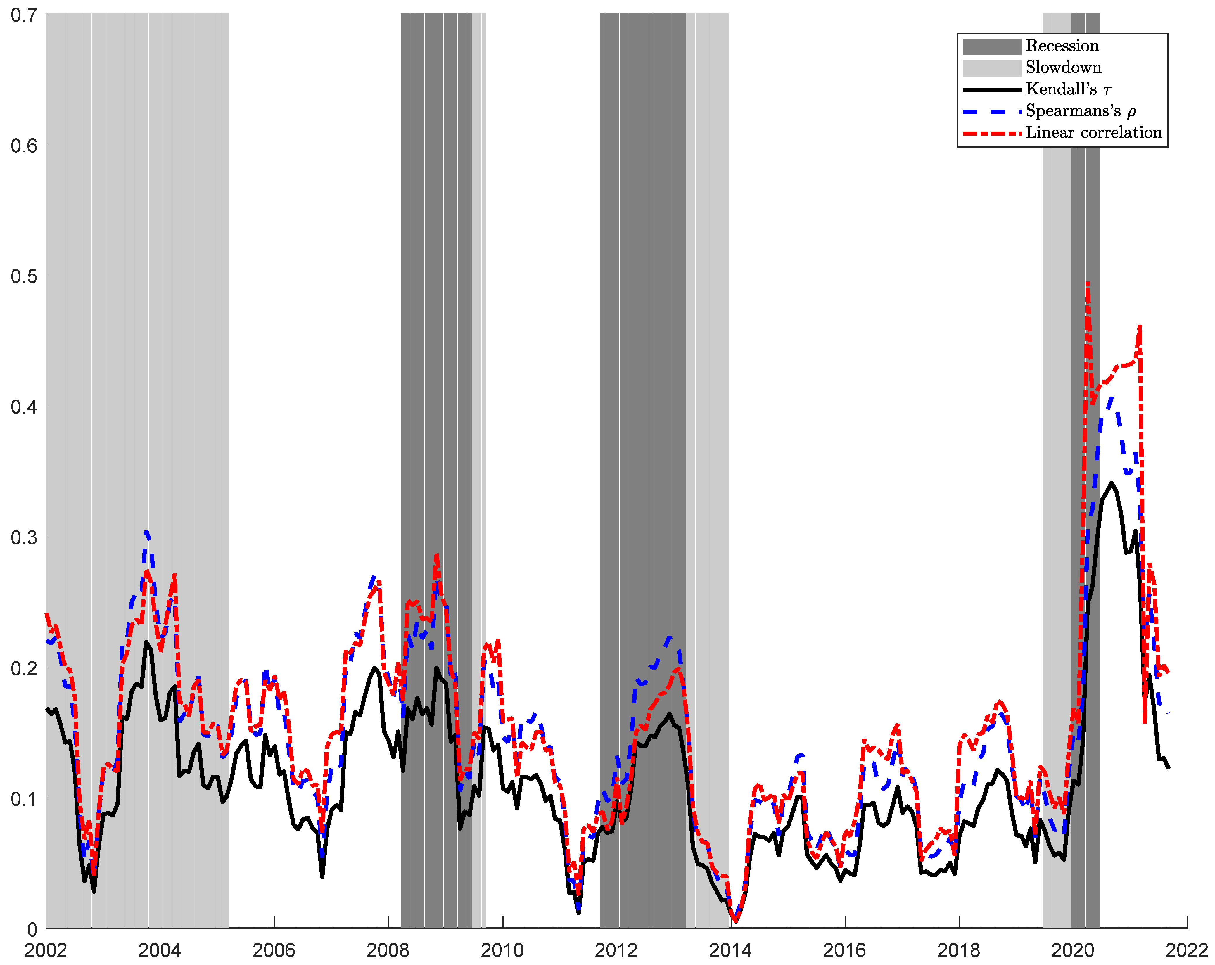
In Figure 1, we compute, using a rolling window of one year, an average over the possible couples of sectors residuals from autoregressive models of the most used measure of bivariate dependence: Linear (Pearson) correlation, Rank Correlation (Spearman’s $\rho$), and Kendall’s $\tau$. Recessions and slowdown periods are from Eurostat’s Business Cycle Clock (BCC). The proposed dependence indicators all increase during recessions. However, we cannot understand if this increase is a statistical fluke due to the small sample. One possible way of formally testing for differences in dependence during a recession is testing the overall radial symmetry of the residual copula. While applying the multiplier bootstrap procedure results in a p-value of 0.8400 and not detecting asymmetry, the randomization procedure produces a p-value of 0.000, strongly suggesting the absence of symmetry. Asymmetry highlights the need for models of the distribution of residuals different from the usual Normal or t-Student assumption.

5. Conclusions

This paper extends the randomization approach in testing radial symmetry in [22] to more than two variables. It also compares in a simulation study with a high number of variables and its computing and statistical performance with the performance of the multiplier bootstrap procedure developed in [19]. However, even if the multiplier approach is computationally advantageous, it is statistically unreliable with a high number of series and observations up to 250. Instead, the randomization approach delivers reasonable size and power with 250 observations and 100 series, particularly for moderate and high values of pairwise Kendall’s tau. Understanding this striking difference in the high dimensional regime would require the study of the asymptotic behavior of the empirical copula process when both n and d go to infinity. This investigation is outside the scope of the paper but would be an exciting avenue for future research. The number of observations is sufficient to investigate asymmetry in a macroeconomic context where the highest frequency of the time series is monthly. Consequently, the samples are much smaller than in a financial application. We apply the randomization test to a European macroeconomic dataset, including growth rates of industrial production in 30 different sectors and 241 observations. Given our simulation study, the rejection of the null of radial symmetry below the 0.01% significance level, a consequence of the smallness of the randomization p-value of the test applied to the industrial production data, has to be considered statistically sounded. To our knowledge, we are the firsts to document radial asymmetry in the joint distribution of the percentage changes of sectorial industrial production indexes of the European Union. This finding allows better models of the joint distribution of the residuals, potentially leading to a better forecast of the economy-wide industrial production. In addition, this detection of asymmetry in industrial production could be a symptom of a change in dependence among sectorial production in recessions and booms, similar to what is happening to asset prices when subject to financial contagion. Those two consequences of our findings will be an exciting avenue for further investigation and research.

References

- Nelsen, R.B. Some concepts of bivariate symmetry. J. Nonparametr. Stat. 1993, 3, 95–101. [Google Scholar] [CrossRef]
- Nelsen, R.B. An Introduction to Copulas, 2nd ed.; Springer Series in Statistics; Springer: New York, NY, USA, 2006. [Google Scholar]
- Longin, F.; Solnik, B. Extreme correlation of international equity markets. J. Financ. 2001, 56, 649–676. [Google Scholar] [CrossRef]
- Ang, A.; Chen, J. Asymmetric correlations of equity portfolios. J. Financ. Econ. 2002, 63, 443–494. [Google Scholar] [CrossRef]
- Billio, M.; Pelizzon, L. Contagion and interdependence in stock markets: Have they been misdiagnosed? J. Econ. Bus. 2003, 55, 405–426. [Google Scholar] [CrossRef]
- Patton, A.J. On the Out-of-Sample Importance of Skewness and Asymmetric Dependence for Asset Allocation. J. Financ. Econom. 2004, 2, 130–168. [Google Scholar] [CrossRef] [Green Version]
- Rémillard, B. Goodness-of-Fit Tests for Copulas of Multivariate Time Series. Econometrics 2017, 5, 13. [Google Scholar] [CrossRef] [Green Version]
- Bücher, A.; Kojadinovic, I. A dependent multiplier bootstrap for the sequential empirical copula process under strong mixing. Bernoulli 2016, 22, 927–968. [Google Scholar] [CrossRef] [Green Version]
- Joe, H. Dependence Modeling with Copulas; Chapman & Hall/CRC Monographs on Statistics & Applied Probability: Boca Raton, FL, USA, 2014. [Google Scholar]
- Durante, F.; Sempi, C. Principles of Copula Theory; CRC Press: Boca Raton, FL, USA, 2015. [Google Scholar]
- Sklar, M. Fonctions de répartition à n dimensions et leurs marges. Publ. Inst. Stat. Univ. Paris 1959, 8, 229–231. [Google Scholar]
- Bouzebda, S.; Cherfi, M. Test of symmetry based on copula function. J. Stat. Plan. Inference 2012, 142, 1262–1271. [Google Scholar] [CrossRef]
- Dehgani, A.; Dolati, A.; Úbeda Flores, M. Measures of radial asymmetry for bivariate random vectors. Stat. Pap. 2013, 54, 271–286. [Google Scholar] [CrossRef]
- Genest, C.; Nešlehová, J.G. On tests of radial symmetry for bivariate copulas. Stat. Pap. 2014, 55, 1107–1119. [Google Scholar] [CrossRef]
- Rosco, J.F.; Joe, H. Measures of tail asymmetry for bivariate copulas. Stat. Pap. 2013, 54, 709–726. [Google Scholar] [CrossRef]
- Li, B.; Genton, M.G. Nonparametric identification of copula structures. J. Am. Stat. Assoc. 2013, 108, 666–675. [Google Scholar] [CrossRef]
- Krupskii, P. Copula-based measures of reflection and permutation asymmetry and statistical tests. Stat. Pap. 2017, 58, 1165–1187. [Google Scholar] [CrossRef]
- Bahraoui, T.; Quessy, J.F. Tests of radial symmetry for multivariate copulas based on the copula characteristic function. Electron. J. Stat. 2017, 11, 2066–2096. [Google Scholar] [CrossRef]
- Billio, M.; Frattarolo, L.; Guégan, D. Multivariate radial symmetry of copula functions: Finite sample comparison in the i.i.d case. Depend. Model. 2021, 9, 43–61. [Google Scholar] [CrossRef]
- Segers, J. Asymptotics of empirical copula processes under non-restrictive smoothness assumptions. Bernoulli 2012, 18, 764–782. [Google Scholar] [CrossRef]
- Quessy, J.F. A general framework for testing homogeneity hypotheses about copulas. Electron. J. Stat. 2016, 10, 1064–1097. [Google Scholar] [CrossRef]
- Beare, B.K.; Seo, J. Randomization test of copula symmetry. Econ. Theory 2020, 36, 1025–1063. [Google Scholar] [CrossRef] [Green Version]
- Kosorok, M. Introduction to Empirical Processes and Semiparametric Inference; Springer Series in Statistics; Springer: New York, NY, USA, 2010. [Google Scholar]
- Hofert, M.; Kojadinovic, I.; Maechler, M.; Yan, J. Copula: Multivariate Dependence with Copulas; R Package Version 1.0-1. 2020. Available online: https://CRAN.R-project.org/package=copula (accessed on 20 November 2021).
- Duchesne, P.; Ghoudi, K.; Rémillard, B. On testing for independence between the innovations of several time series. Can. J. Stat. 2012, 40, 447–479. [Google Scholar] [CrossRef]
- Bucher, A.; Jaschke, S.; Wied, D. Nonparametric tests for constant tail dependence with an application to energy and finance. J. Econom. 2015, 187, 154–168. [Google Scholar] [CrossRef]
- Nasri, B.R.; Rémillard, B.N.; Bahraoui, T. Change-point problems for multivariate time series using pseudo-observations. J. Multivar. Anal. 2022, 187, 104857. [Google Scholar] [CrossRef]
- Pollard, D. Empirical Processes: Theory and Applications; Conference Board of the Mathematical Science: NSF-CBMS Regional Conference Series in Probability and Statistics; Institute of Mathematical Statistics: Hayward, CA, USA, 1990. [Google Scholar]
- Bücher, A.; Volgushev, S. Empirical and sequential empirical copula processes under serial dependence. J. Multivar. Anal. 2013, 119, 61–70. [Google Scholar] [CrossRef]
Figure 1.
Average Linear correlation, Spearman’s , and Kendall’s , computed using a rolling window of one year. Recessions and slowdown periods are from Eurostat’s Business Cycle Clock (BCC).