
Water Mass Transport Changes through the Venice Lagoon Inlets from Projected Sea-Level Changes under a Climate Warming Scenario
 , , , , ,
Abstract
:1. Introduction
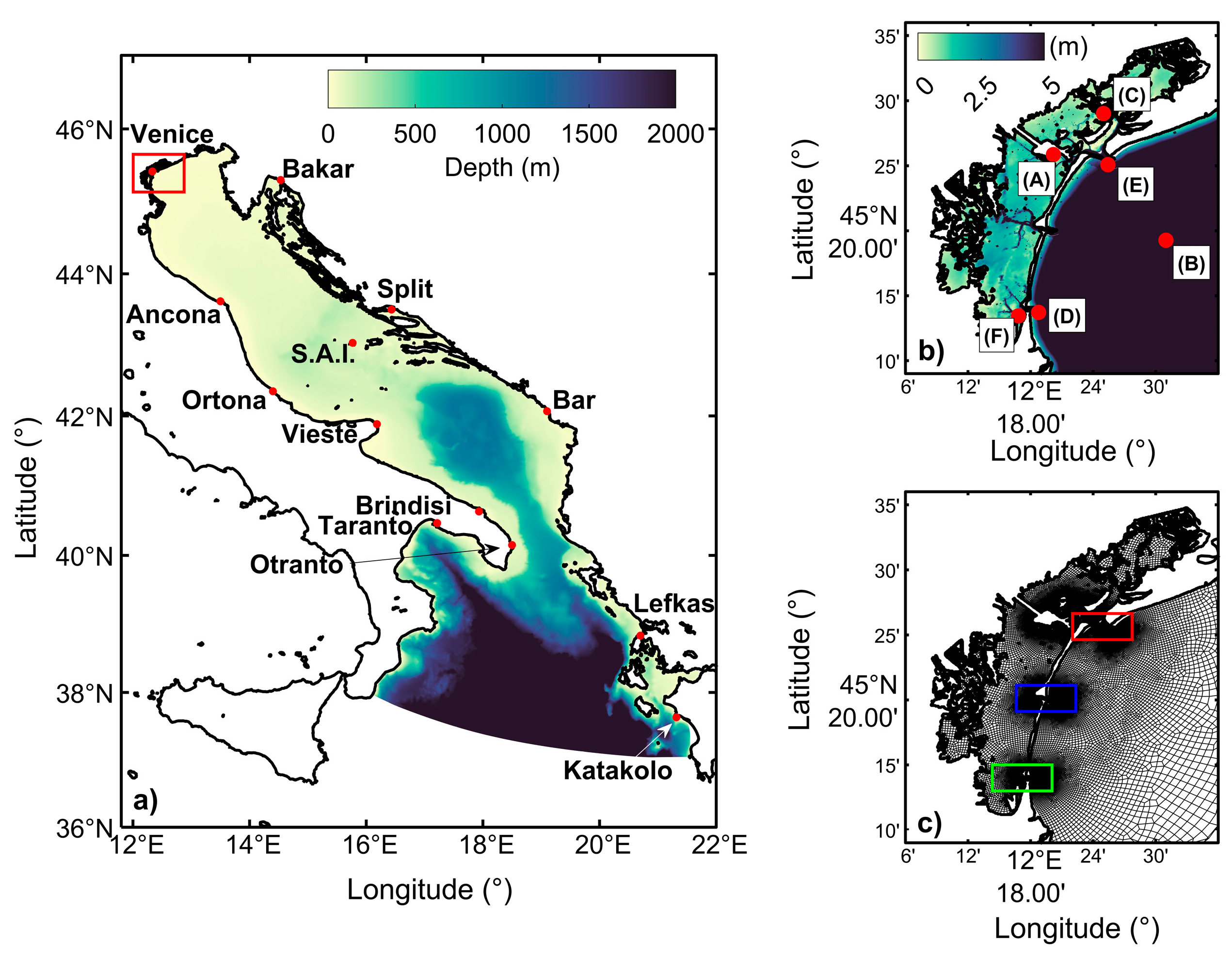
2. Study Site

| Site | LAT | LON | M2 | S2 | K1 | O1 | ||||||||||||||||
|---|---|---|---|---|---|---|---|---|---|---|---|---|---|---|---|---|---|---|---|---|---|---|
| Ao (cm) | As (cm) | θo (°) | θs (°) | d (cm) | Ao (cm) | As (cm) | θo (°) | θs (°) | d (cm) | Ao (cm) | As (cm) | θo (°) | θs (°) | d (cm) | Ao (cm) | As (cm) | θo (°) | θs (°) | d (cm) | |||
| Venice | 45°25′ | 12°20′ | 23.4 | 21.1 | 259 | 264 | 3.0 | 14.1 | 14.4 | 265 | 268 | 0.8 | 17.9 | 17.8 | 61 | 41 | 6.2 | 5.6 | 4.4 | 50 | 22 | 2.7 |
| Bakar | 45°18′ | 14°32′ | 10.6 | 9.4 | 208 | 207 | 1.2 | 5.5 | 6.1 | 2.2 | 205 | 0.9 | 13.8 | 14.9 | 48 | 22 | 6.5 | 4.1 | 3.8 | 38 | 4 | 2.3 |
| Ancona | 43°37′ | 13°30′ | 6.6 | 5.0 | 302 | 292 | 1.9 | 3.6 | 2.7 | 315 | 308 | 1.0 | 13 | 12.8 | 72 | 42 | 6.7 | 4.2 | 3.3 | 61 | 22 | 2.6 |
| Split | 43°30′ | 16°26′ | 8 | 8.0 | 100 | 80 | 2.8 | 5.6 | 6.1 | 100 | 78 | 2.3 | 8.8 | 8.9 | 41 | 12 | 4.4 | 2.7 | 2.5 | 34 | 356 | 1.7 |
| S.A.I. | 43°02′ | 15°46′ | 6.8 | 6.5 | 93 | 73 | 2.3 | 4.4 | 5.0 | 95 | 72 | 1.9 | 6.8 | 8.4 | 54 | 22 | 4.5 | 2.5 | 2.3 | 42 | 4 | 1.6 |
| Ortona | 42°21′ | 14°24′ | 6.4 | 6.1 | 64 | 55 | 1.0 | 4.5 | 4.7 | 76 | 58 | 1.5 | 9.7 | 8.9 | 73 | 39 | 5.5 | 3.4 | 2.5 | 53 | 18 | 2.0 |
| Vieste | 41°53′ | 16°11′ | 7.9 | 8.1 | 61 | 59 | 0.2 | 5.1 | 5.8 | 83 | 62 | 2.1 | 4.2 | 5.0 | 65 | 46 | 1.7 | 1.5 | 1.7 | 52 | 25 | 0.7 |
| Bar | 42°04′ | 19°06′ | 9.2 | 8.6 | 76 | 61 | 2.4 | 5.6 | 5.9 | 80 | 61 | 1.9 | 4.8 | 5.3 | 42 | 16 | 2.3 | 1.4 | 1.7 | 19 | 359 | 0.6 |
| Brindisi | 40°38′ | 17°56′ | 8.7 | 7.9 | 73 | 65 | 1.4 | 5.2 | 5.3 | 81 | 67 | 1.3 | 4.6 | 5.0 | 54 | 34 | 1.7 | 1.5 | 1.6 | 43 | 12 | 0.8 |
| Otranto | 40°09′ | 18°30′ | 7 | 6.4 | 74 | 65 | 1.2 | 4 | 3.9 | 82 | 66 | 1.1 | 2.3 | 3.1 | 64 | 36 | 1.5 | 1.0 | 1.2 | 44 | 13 | 0.6 |
| Lefkas | 38°50′ | 20°42′ | 4 | 4.6 | 79 | 54 | 2.0 | 2.2 | 2.7 | 85 | 52 | 1.5 | 1.4 | 2.1 | 19 | 6 | 0.8 | 0.6 | 0.9 | 5 | 254 | 0.3 |
| Katakolo | 37°38′ | 21°19′ | 3.3 | 3.4 | 62 | 53 | 0.5 | 1.6 | 2.0 | 65 | 48 | 0.6 | 1.3 | 1.7 | 6 | 1 | 0.4 | 0.5 | 0.7 | 353 | 347 | 0.2 |
| Taranto | 40°28′ | 17°13′ | 6.5 | 5.2 | 71 | 59 | 1.8 | 3.7 | 3.0 | 73 | 59 | 1.1 | 1.8 | 2.3 | 42 | 22 | 0.9 | 0.8 | 1.0 | 34 | 5 | 0.5 |
| RMS (cm) | 1.3 | 1.0 | 2.8 | 1.1 | ||||||||||||||||||
3. Numerical Experiments and Model Setup
3.1. Mesh and Bathymetry
3.2. Experimental Design
3.3. Boundary Forcing
3.3.1. Atmospheric Forcing
3.3.2. Open Ocean Boundary
4. Results and Discussion
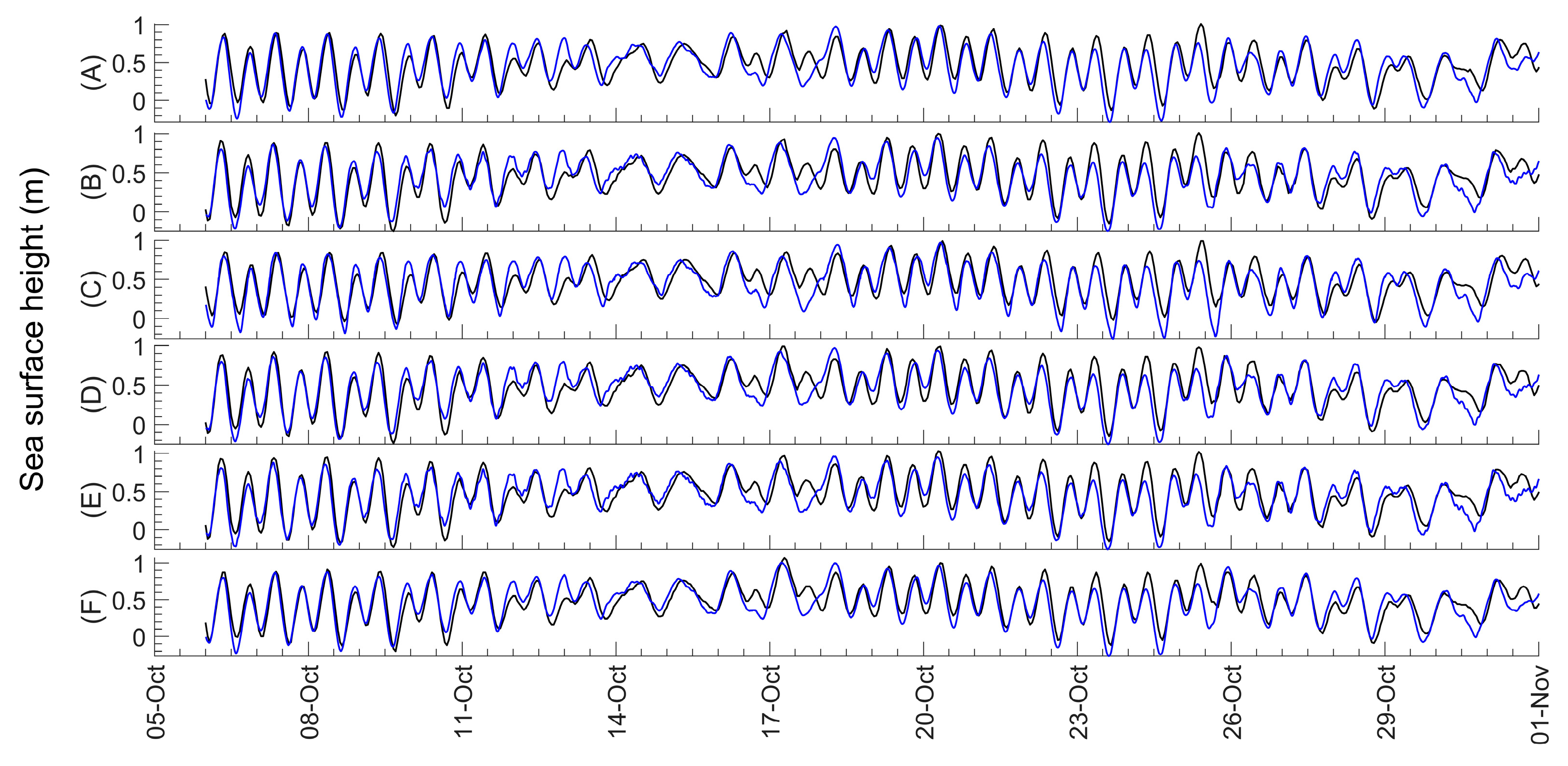
4.1. Model Performance and Biases
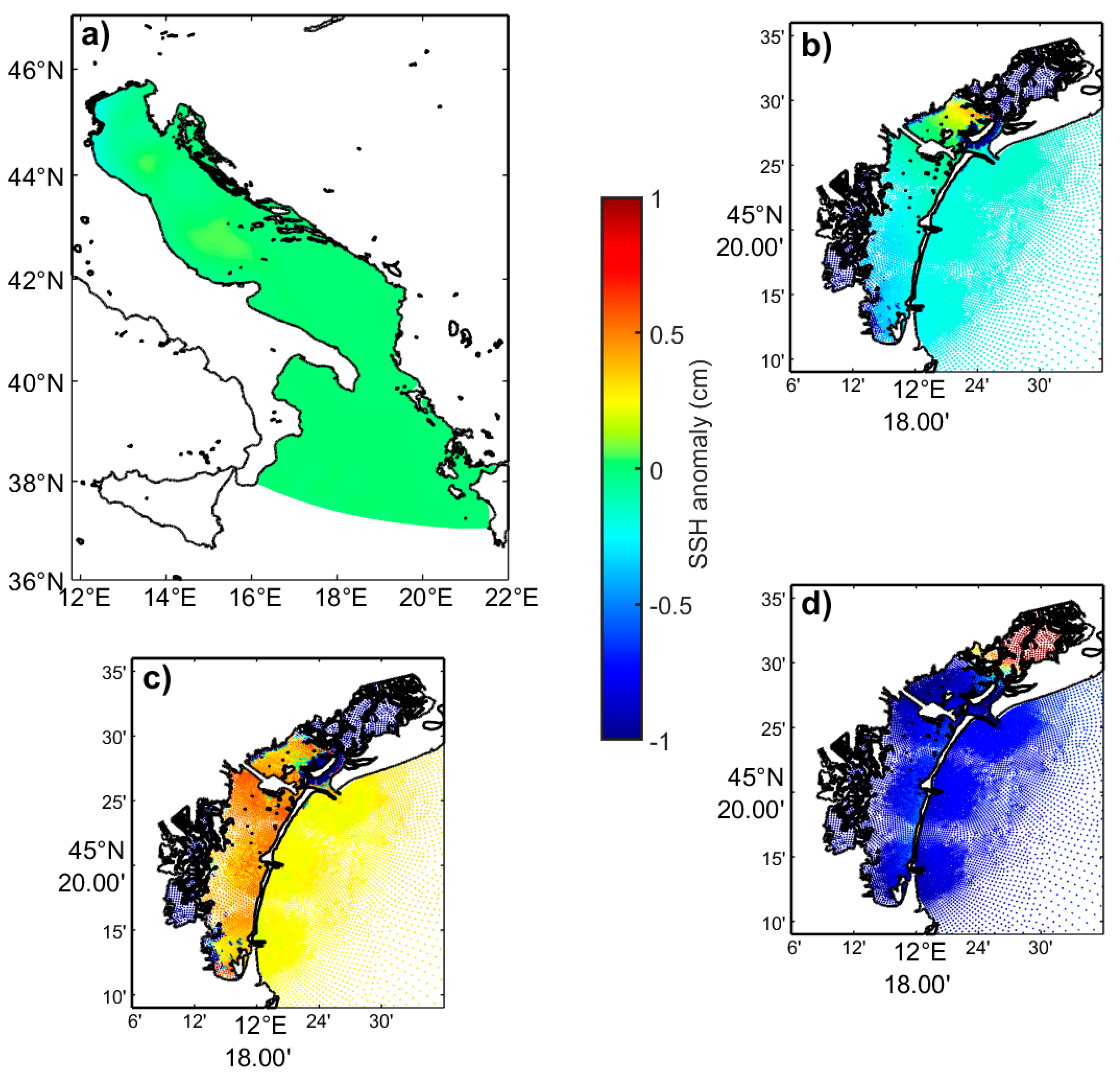
4.2. Sea Level Rise in the Adriatic Sea and inside the Venice Lagoon
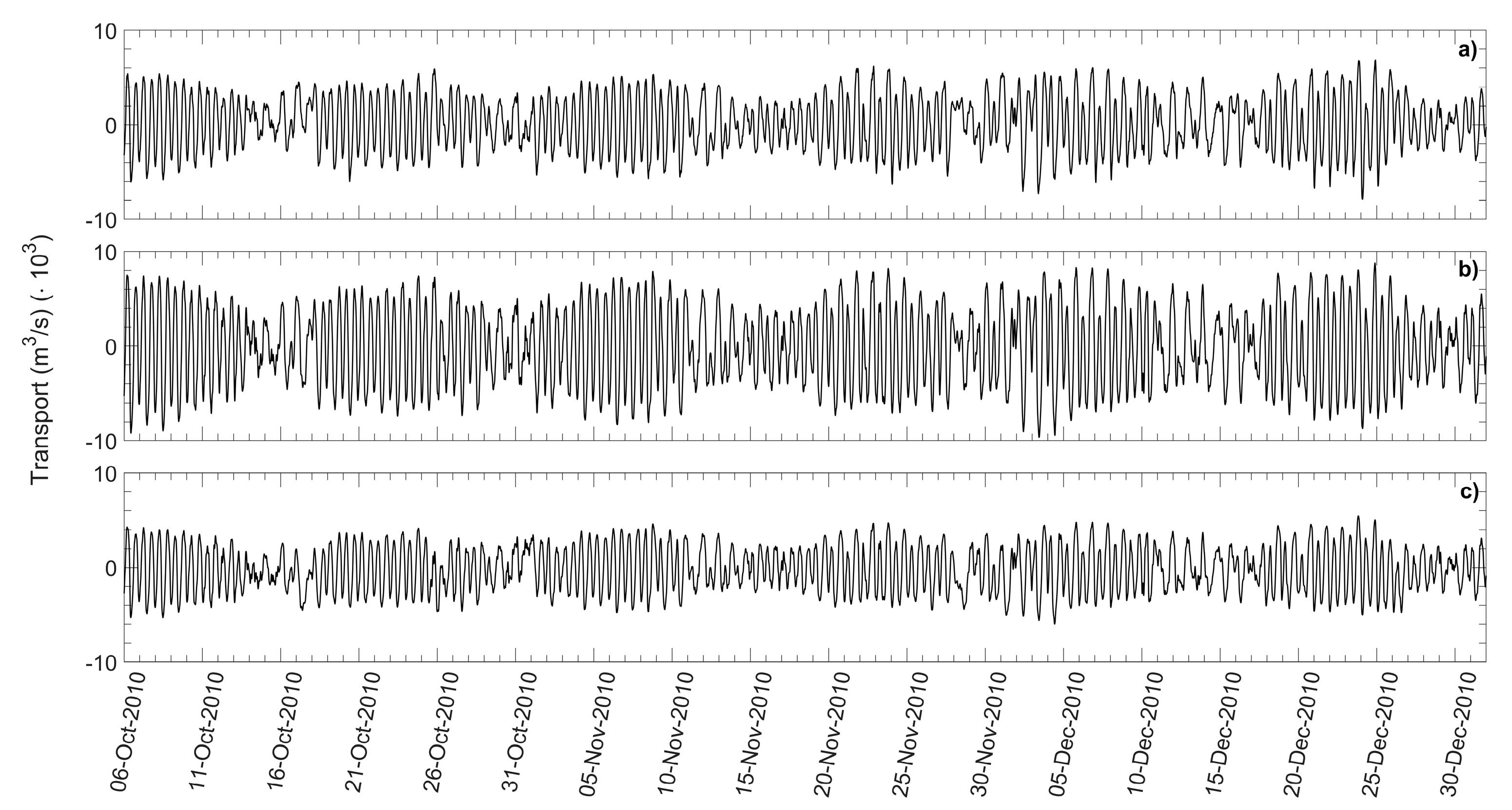
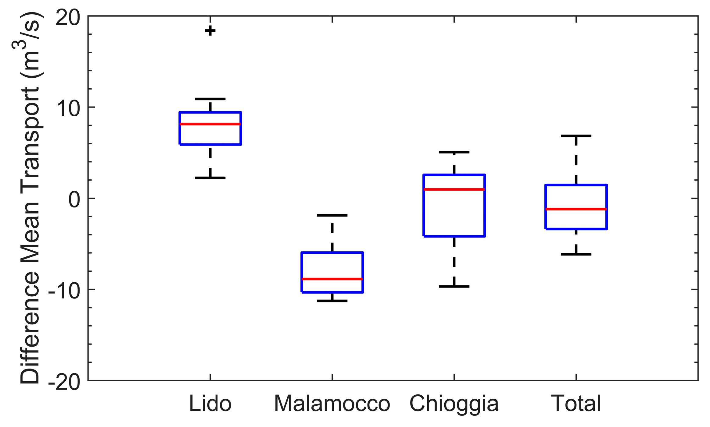
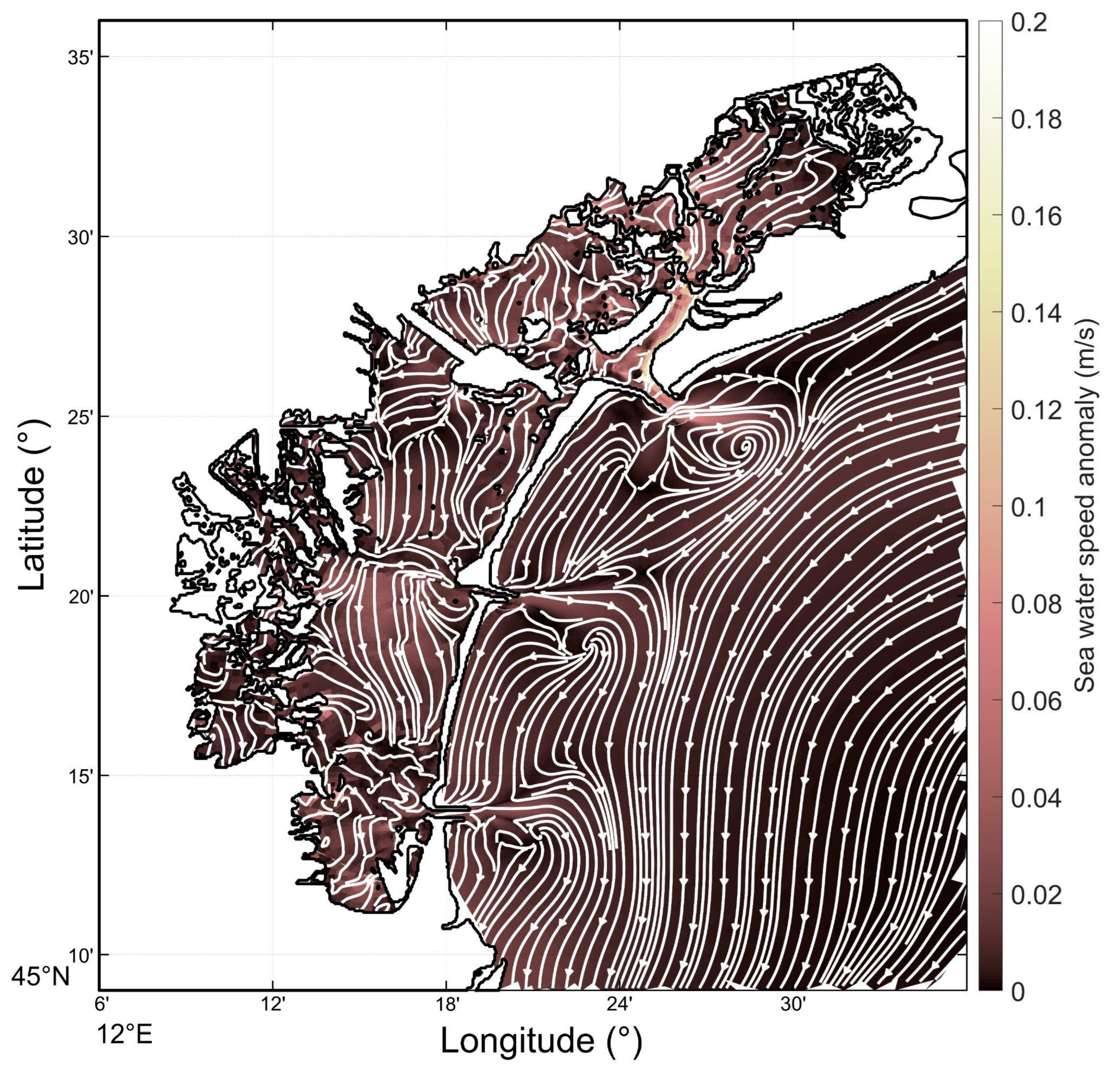
4.3. Water Mass Exchanges between the Lagoon and the Open Sea
5. Conclusions
Author Contributions
Funding
Data Availability Statement
Acknowledgments
Conflicts of Interest
References
- Pham, H.V.; Dal Barco, M.K.; Cadau, M.; Harris, R.; Furlan, E.; Torresan, S.; Rubinetti, S.; Zanchettin, D.; Rubino, A.; Kuznetsov, I.; et al. Multi-Model Chain for Climate Change Scenario Analysis to Support Coastal Erosion and Water Quality Risk Management for the Metropolitan City of Venice. Sci. Total Environ. 2023, 904, 166310. [Google Scholar] [CrossRef]
- Zanchettin, D.; Bruni, S.; Raicich, F.; Lionello, P.; Adloff, F.; Androsov, A.; Antonioli, F.; Artale, V.; Carminati, E.; Ferrarin, C.; et al. Sea-Level Rise in Venice: Historic and Future Trends (Review Article). Nat. Hazards Earth Syst. Sci. 2021, 21, 2643–2678. [Google Scholar] [CrossRef]
- Rubinetti, S.; Taricco, C.; Zanchettin, D.; Arnone, E.; Bizzarri, I.; Rubino, A. Interannual-to-Multidecadal Sea-Level Changes in the Venice Lagoon and Their Impact on Flood Frequency. Clim. Chang. 2022, 174, 26. [Google Scholar] [CrossRef]
- Zanchettin, D.; Rubinetti, S.; Rubino, A. Is the Atlantic a Source for Decadal Predictability of Sea-Level Rise in Venice? Earth Space Sci. 2022, 9, e2022EA002494. [Google Scholar] [CrossRef]
- MOSE Venezia Project MOSE Venezia|Project 2022. Available online: https://www.mosevenezia.eu/project/?lang=en (accessed on 9 September 2023).
- Umgiesser, G. The Impact of Operating the Mobile Barriers in Venice (MOSE) under Climate Change. J. Nat. Conserv. 2020, 54, 125783. [Google Scholar] [CrossRef]
- Lionello, P.; Nicholls, R.J.; Umgiesser, G.; Zanchettin, D. Venice Flooding and Sea Level: Past Evolution, Present Issues, and Future Projections (Introduction to the Special Issue). Nat. Hazards Earth Syst. Sci. 2021, 21, 2633–2641. [Google Scholar] [CrossRef]
- Tognin, D.; D’Alpaos, A.; Marani, M.; Carniello, L. Marsh Resilience to Sea-Level Rise Reduced by Storm-Surge Barriers in the Venice Lagoon. Nat. Geosci. 2021, 14, 906–911. [Google Scholar] [CrossRef]
- Scarpa, G.M.; Braga, F.; Manfè, G.; Lorenzetti, G.; Zaggia, L. Towards an Integrated Observational System to Investigate Sediment Transport in the Tidal Inlets of the Lagoon of Venice. Remote Sens. 2022, 14, 3371. [Google Scholar] [CrossRef]
- Anelli Monti, M.; Brigolin, D.; Franzoi, P.; Libralato, S.; Pastres, R.; Solidoro, C.; Zucchetta, M.; Pranovi, F. Ecosystem Functioning and Ecological Status in the Venice Lagoon, Which Relationships? Ecol. Indic. 2021, 133, 108461. [Google Scholar] [CrossRef]
- Tsimplis, M.N.; Marcos, M.; Somot, S. 21st Century Mediterranean Sea Level Rise: Steric and Atmospheric Pressure Contributions from a Regional Model. Glob. Planet. Chang. 2008, 63, 105–111. [Google Scholar] [CrossRef]
- Ferrarin, C.; Tomasin, A.; Bajo, M.; Petrizzo, A.; Umgiesser, G. Tidal Changes in a Heavily Modified Coastal Wetland. Cont. Shelf Res. 2015, 101, 22–33. [Google Scholar] [CrossRef]
- Benetazzo, A.; Davison, S.; Barbariol, F.; Mercogliano, P.; Favaretto, C.; Sclavo, M. Correction of ERA5 Wind for Regional Climate Projections of Sea Waves. Water 2022, 14, 1590. [Google Scholar] [CrossRef]
- Umgiesser, G.; Bajo, M.; Ferrarin, C.; Cucco, A.; Lionello, P.; Zanchettin, D.; Papa, A.; Tosoni, A.; Ferla, M.; Coraci, E.; et al. The Prediction of Floods in Venice: Methods, Models and Uncertainty (Review Article). Nat. Hazards Earth Syst. Sci. 2021, 21, 2679–2704. [Google Scholar] [CrossRef]
- Cavaleri, L.; Bajo, M.; Barbariol, F.; Bastianini, M.; Benetazzo, A.; Bertotti, L.; Chiggiato, J.; Davolio, S.; Ferrarin, C.; Magnusson, L.; et al. The October 29, 2018 Storm in Northern Italy—An Exceptional Event and Its Modeling. Prog. Oceanogr. 2019, 178, 102178. [Google Scholar] [CrossRef]
- Vilibić, I.; Šepić, J.; Pasarić, M.; Orlić, M. The Adriatic Sea: A Long-Standing Laboratory for Sea Level Studies. Pure Appl. Geophys. 2017, 174, 3765–3811. [Google Scholar] [CrossRef]
- Tsimplis, M.N.; Proctor, R.; Flather, R.A. A Two-Dimensional Tidal Model for the Mediterranean Sea. J. Geophys. Res. Oceans 1995, 100, 16223–16239. [Google Scholar] [CrossRef]
- Androsov, A.; Fofonova, V.; Kuznetsov, I.; Danilov, S.; Rakowsky, N.; Harig, S.; Brix, H.; Wiltshire, K.H. FESOM-C v.2: Coastal Dynamics on Hybrid Unstructured Meshes. Geosci. Model Dev. 2019, 12, 1009–1028. [Google Scholar] [CrossRef]
- Fofonova, V.; Androsov, A.; Sander, L.; Kuznetsov, I.; Amorim, F.; Hass, H.C.; Wiltshire, K.H. Non-Linear Aspects of the Tidal Dynamics in the Sylt-Rømø Bight, South-Eastern North Sea. Ocean Sci. 2019, 15, 1761–1782. [Google Scholar] [CrossRef]
- Kuznetsov, I.; Androsov, A.; Fofonova, V.; Danilov, S.; Rakowsky, N.; Harig, S.; Wiltshire, K.H. Evaluation and Application of Newly Designed Finite Volume Coastal Model FESOM-C, Effect of Variable Resolution in the Southeastern North Sea. Water 2020, 12, 1412. [Google Scholar] [CrossRef]
- Debolskaya, E.I.; Kuznetsov, I.S.; Androsov, A.A. Numerical Simulation of Hydrodynamic Processes in Indiga Bay. Power Technol. Eng. 2023, 56, 691–697. [Google Scholar] [CrossRef]
- Neder, C.; Fofonova, V.; Androsov, A.; Kuznetsov, I.; Abele, D.; Falk, U.; Schloss, I.R.; Sahade, R.; Jerosch, K. Modelling Suspended Particulate Matter Dynamics at an Antarctic Fjord Impacted by Glacier Melt. J. Mar. Syst. 2022, 231, 103734. [Google Scholar] [CrossRef]
- Remacle, J.-F.; Lambrechts, J.; Seny, B.; Marchandise, E.; Johnen, A.; Geuzainet, C. Blossom-Quad: A Non-Uniform Quadrilateral Mesh Generator Using a Minimum-Cost Perfect-Matching Algorithm. Int. J. Numer. Methods Eng. 2012, 89, 1102–1119. [Google Scholar] [CrossRef]
- Geuzaine, C.; Remacle, J.-F. Gmsh: A 3-D Finite Element Mesh Generator with Built-in Pre- and Post-Processing Facilities. Int. J. Numer. Methods Eng. 2009, 79, 1309–1331. [Google Scholar] [CrossRef]
- EMODnet Bathymetry Consortium EMODnet Digital Bathymetry (DTM). 2020. Available online: https://sextant.ifremer.fr/record/bb6a87dd-e579-4036-abe1-e649cea9881a/ (accessed on 9 September 2023).
- Madricardo, F.; Foglini, F.; Trincardi, F. Processed High-Resolution ASCII:ESRI Gridded Bathymetry Data (EM2040 and EM3002) from the Lagoon of Venice Collected in 2013. Available online: https://www.marine-geo.org/tools/search/Files.php?data_set_uid=23605 (accessed on 9 September 2023).
- Wessel, P.; Smith, W.H. A Global, Self-Consistent, Hierarchical, High-Resolution Shoreline Database. J. Geophys. Res. Solid Earth 1996, 101, 8741–8743. [Google Scholar] [CrossRef]
- Hersbach, H.; Bell, B.; Berrisford, P.; Hirahara, S.; Horányi, A.; Muñoz-Sabater, J.; Nicolas, J.; Peubey, C.; Radu, R.; Schepers, D.; et al. The ERA5 Global Reanalysis. Q. J. R. Meteorol. Soc. 2020, 146, 1999–2049. [Google Scholar] [CrossRef]
- CDS ERA5 Hourly Data on Single Levels from 1959 to Present. Available online: https://cds.climate.copernicus.eu/cdsapp#!/dataset/reanalysis-era5-single-levels?tab=overview (accessed on 9 September 2023).
- Rockel, B.; Will, A.; Hense, A. The Regional Climate Model COSMO-CLM (CCLM). Meteorol. Z. 2008, 17, 347–348. [Google Scholar] [CrossRef]
- Egbert, G.D.; Erofeeva, S.Y. Efficient Inverse Modeling of Barotropic Ocean Tides. J. Atmos. Ocean. Technol. 2002, 19, 183–204. [Google Scholar] [CrossRef]
- Egbert, G.D.; Bennett, A.F.; Foreman, M.G.G. TOPEX/POSEIDON Tides Estimated Using a Global Inverse Model. J. Geophys. Res. Oceans 1994, 99, 24821–24852. [Google Scholar] [CrossRef]
- OSU TPXO Tide Models OSU TPXO Tide Models—TPXO9-Atlas. Available online: https://www.tpxo.net/global/tpxo9-atlas (accessed on 31 May 2022).
- Pawlowicz, R.; Beardsley, B.; Lentz, S. Classical Tidal Harmonic Analysis Including Error Estimates in MATLAB Using T_TIDE. Comput. Geosci. 2002, 28, 929–937. [Google Scholar] [CrossRef]
- Yan, K.; Muis, S.; Irazoqui, M.; Verlaan, M. ‘Water Level Change Time Series for the European Coast from 1977 to 2100 Derived from Climate Projections’. Copernicus Climate Change Service (C3S) Climate Data Store (CDS). 2020. Available online: https://cds.climate.copernicus.eu/cdsapp#!/dataset/sis-water-level-change-timeseries?tab=overview (accessed on 9 September 2023).
- Lionello, P.; Barriopedro, D.; Ferrarin, C.; Nicholls, R.J.; Orlić, M.; Raicich, F.; Reale, M.; Umgiesser, G.; Vousdoukas, M.; Zanchettin, D. Extreme Floods of Venice: Characteristics, Dynamics, Past and Future Evolution (Review Article). Nat. Hazards Earth Syst. Sci. 2021, 21, 2705–2731. [Google Scholar] [CrossRef]
- Foreman, M.G.G.; Henry, R.F.; Walters, R.A.; Ballantyne, V.A. A Finite Element Model for Tides and Resonance along the North Coast of British Columbia. J. Geophys. Res. Oceans 1993, 98, 2509–2531. [Google Scholar] [CrossRef]
- CPSM Centro Previsioni e Segnalazioni Maree Website—The Tide. Available online: https://www.comune.venezia.it/it/content/la-marea (accessed on 16 March 2022).
- Cavaleri, L.; Bertotti, L. Accuracy of the Modelled Wind and Wave Fields in Enclosed Seas. Tellus A Dyn. Meteorol. Oceanogr. 2004, 56, 167–175. [Google Scholar] [CrossRef]
- Gačić, M.; Kovačević, V.; Mazzoldi, A.; Paduan, J.; Arena, F.; Mosquera, I.M.; Gelsi, G.; Arcari, G. Measuring Water Exchange between the Venetian Lagoon and the Open Sea. Eos Trans. Am. Geophys. Union 2002, 83, 217–222. [Google Scholar] [CrossRef]


| 2000 | 2001 | 2002 | 2003 | 2004 | 2005 | 2006 | 2007 | 2008 | 2009 | 2010 | |
|---|---|---|---|---|---|---|---|---|---|---|---|
| A | 17.6 | 22.7 | 18.4 | 20.6 | 17.8 | 17.8 | 17.1 | 18.9 | 18.8 | 18.5 | 19.3 |
| B | 16.9 | 22.5 | 17.9 | 20.0 | 17.3 | 17.3 | 16.3 | 18.8 | 17.5 | 17.4 | 17.9 |
| C | - | - | - | 19.4 | 19.9 | 17.7 | 16.4 | 19.2 | 18.4 | 18.0 | 18.7 |
| D | 16.5 | 22.5 | 17.9 | 20.0 | 17.3 | 17.1 | 16.2 | 18.2 | 18.0 | 17.1 | 17.8 |
| E | 17.2 | 21.9 | 18.2 | 20.1 | 17.3 | 17.3 | 16.3 | 18.5 | 18.1 | 17.6 | 18.3 |
| F | 17.3 | 19.9 | 18.2 | 20.5 | 17.5 | 17.6 | 17.0 | 19.2 | 18.1 | 17.9 | 18.0 |
Disclaimer/Publisher’s Note: The statements, opinions and data contained in all publications are solely those of the individual author(s) and contributor(s) and not of MDPI and/or the editor(s). MDPI and/or the editor(s) disclaim responsibility for any injury to people or property resulting from any ideas, methods, instructions or products referred to in the content. |
© 2023 by the authors. Licensee MDPI, Basel, Switzerland. This article is an open access article distributed under the terms and conditions of the Creative Commons Attribution (CC BY) license (https://creativecommons.org/licenses/by/4.0/).
Share and Cite
Rubinetti, S.; Kuznetsov, I.; Fofonova, V.; Androsov, A.; Gnesotto, M.; Rubino, A.; Zanchettin, D. Water Mass Transport Changes through the Venice Lagoon Inlets from Projected Sea-Level Changes under a Climate Warming Scenario. Water 2023, 15, 3221. https://doi.org/10.3390/w15183221
Rubinetti S, Kuznetsov I, Fofonova V, Androsov A, Gnesotto M, Rubino A, Zanchettin D. Water Mass Transport Changes through the Venice Lagoon Inlets from Projected Sea-Level Changes under a Climate Warming Scenario. Water. 2023; 15(18):3221. https://doi.org/10.3390/w15183221
Chicago/Turabian StyleRubinetti, Sara, Ivan Kuznetsov, Vera Fofonova, Alexey Androsov, Michele Gnesotto, Angelo Rubino, and Davide Zanchettin. 2023. "Water Mass Transport Changes through the Venice Lagoon Inlets from Projected Sea-Level Changes under a Climate Warming Scenario" Water 15, no. 18: 3221. https://doi.org/10.3390/w15183221